
Open-Source Internship opportunity by OpenGenus for programmers. Apply now.
Reading time: 35 minutes | Coding time: 10 minutes
What is Histogram of Oreinted Gradients (HOG)?
Navneet Dalal and Bill Triggs introduced Histogram of Oriented Gradients(HOG) features in 2005. Histogram of Oriented Gradients (HOG) is a feature descriptor used in image processing, mainly for object detection. A feature descriptor is a representation of an image or an image patch that simplifies the image by extracting useful information from it.
The principle behind the histogram of oriented gradients descriptor is that local object appearance and shape within an image can be described by the distribution of intensity gradients or edge directions. The x and y derivatives of an image (Gradients) are useful because the magnitude of gradients is large around edges and corners due to abrupt change in intensity and we know that edges and corners pack in a lot more information about object shape than flat regions. So, the histograms of directions of gradients are used as features in this descriptor.
Workflow of object detection using HOG
Now that we know basic priciple of Histogram of Oriented Gradients we will be moving into how we calculate the histograms and how these feature vectors, that are obtained from the HOG descriptor, are used by the classifier such a SVM to detect the concerned object.
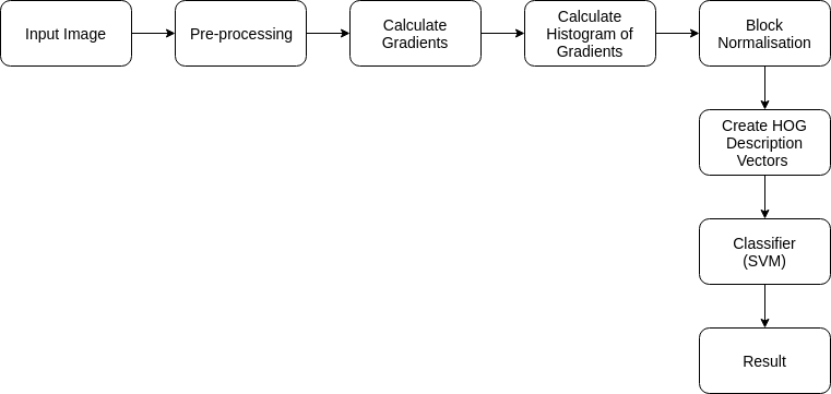 Steps for Object Detection with HOG
How Histogram of Oreinted Gradients(HOG) Works?
Pre-processing
Preprocessing of image involves normalising the image but it is entirely optional. It is used to improve performance of the HOG descriptor. Since, here we are building a simple descriptor we don't use any normalisation in preprocessing.
Computing Gradient
The first actual step in the HOG descriptor is to compute the image gradient in both the x and y direction.
Let us take an example. Say the pixel Q has values surrounding it as shown below:
We can calculate the Gradient magnitude for Q in x and y direction as follow:
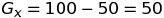
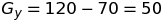
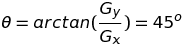
We can get the magnitude of the gradient as:
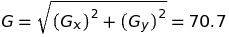
And the direcction of the gradient as :
Compute Histogram of Gradients in 8×8 cells
- The image is divided into 8×8 cell blocks and a histogram of gradients is calculated for each 8×8 cell block.
- The histogram is essentially a vector of 9 buckets ( numbers ) corresponding to angles from 0 to 180 degree (20 degree increments).
- The values of these 64 cells (8X8) are binned and cumulatively added into these 9 buckets.
- This essentially reduces 64 values into 9 values.
A great illustration of this is shown on learnopencv. The following figure shows how it is done. The blue pixel encircled has an angle of 80 degrees and magnitude of 2. So it adds 2 to the 5th bin. The gradient at the pixel encircled using red has an angle of 10 degrees and magnitude of 4. Since 10 degrees is half way between 0 and 20, the vote by the pixel splits evenly into the two bins.
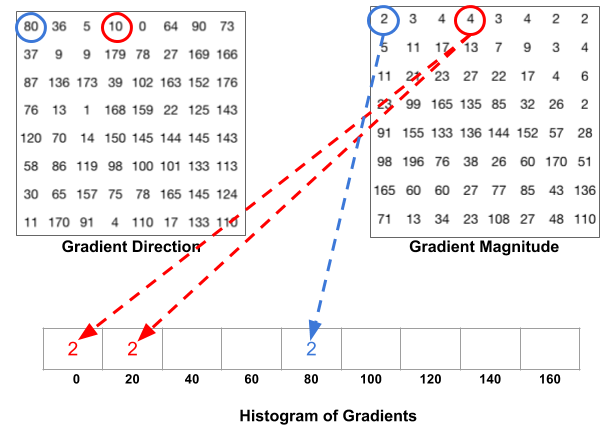
Illustration of splitting of gradient magitude according to gradient direction (Image source: https://www.learnopencv.com/histogram-of-oriented-gradients)
Block Normalization
After the creation of histogram of oriented gradients we need to something else too. Gradient is sensitive to overall lighting. If we say divide/multiply pixel values by some constant in order to make it lighter/ darker the gradient magnitude will change and so will histogram values. We want that histogram values be independent of lighting. Normalization is done on the histogram vector v within a block. One of the following norms could be used:
- L1 norm
- L2 norm
- L2-Hys(Lowe-style clipped L2 norm)
Now, we could simply normalize the 9×1 histogram vector but it is better to normalize a bigger sized block of 16×16. A 16×16 block has 4 histograms (8×8 cell results to one histogram) which can be concatenated to form a 36 x 1 element vector and normalized. The 16×16 window then moves by 8 pixels and a normalized 36×1 vector is calculated over this window and the process is repeated for the image.
Calculate HOG Descriptor vector
-
To calculate the final feature vector for the entire image patch, the 36×1 vectors are concatenated into one giant vector.
-
So, say if there was an input picture of size 64×64 then the 16×16 block has 7 positions horizontally and 7 position vertically.
-
In one 16×16 block we have 4 histograms which after normalization concatinate to form a 36×1 vector.
-
This block moves 7 positions horizontally and vertically totalling it to 7×7 = 49 positions.
-
So when we concatenate them all into one gaint vector we obtain a 36×49 = 1764 dimensional vector.
This vector is now used to train classifiers such as SVM and then do object detection.
Visualization of HOG features
Here is a snippet to visualise HOG features of an Image provided in Scikit-Image's docs to visualize HOG features.
import matplotlib.pyplot as plt

from skimage.feature import hog
from skimage import data, exposure


image = data.astronaut()

fd, hog_image = hog(image, orientations=8, pixels_per_cell=(16, 16),
                    cells_per_block=(1, 1), visualize=True, multichannel=True)

fig, (ax1, ax2) = plt.subplots(1, 2, figsize=(12, 6), sharex=True, sharey=True)

ax1.axis('off')
ax1.imshow(image, cmap=plt.cm.gray)
ax1.set_title('Input image')

# Rescale histogram for better display
hog_image_rescaled = exposure.rescale_intensity(hog_image, in_range=(0, 10))

ax2.axis('off')
ax2.imshow(hog_image_rescaled, cmap=plt.cm.gray)
ax2.set_title('Histogram of Oriented Gradients')
plt.show()
Output as follow:
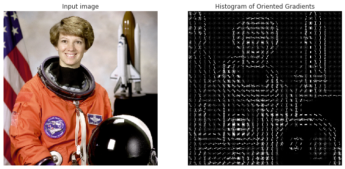
Visualization of HOG features of image of the astronaut Eileen Collins.
Implementation
In this tutorial we will be performing a simple Face Detection using HOG features.
We need to first train the classifier in order to do face detection so first we will need to have training set for the classifier.
Training Set
- Positive training samples
Labeled Faces in the Wild dataset provided by Scikit-Learn consists of variety of faces which is perfect for our positive set.
from sklearn.datasets import fetch_lfw_people
faces = fetch_lfw_people()
positive_patches = faces.images
- Negative training samples
For Negative set we need images without face on them. Scikit-Image offers images which can be used in this case. To incerease the size of negative set we extract patches of image at different scale using PatchExtractor from Scikit-Learn.
from skimage import data, transform
from sklearn.feature_extraction.image import PatchExtractor

imgs_to_use = ['camera', 'text', 'coins', 'moon',
               'page', 'clock', 'immunohistochemistry',
               'chelsea', 'coffee', 'hubble_deep_field']
images = [color.rgb2gray(getattr(data, name)())
          for name in imgs_to_use]


def extract_patches(img, N, scale=1.0, patch_size=positive_patches[0].shape):
    extracted_patch_size = tuple((scale * np.array(patch_size)).astype(int))
    extractor = PatchExtractor(patch_size=extracted_patch_size,
                               max_patches=N, random_state=0)
    patches = extractor.transform(img[np.newaxis])
    if scale != 1:
        patches = np.array([transform.resize(patch, patch_size)
                            for patch in patches])
    return patches

negative_patches = np.vstack([extract_patches(im, 1000, scale)
                              for im in images for scale in [0.5, 1.0, 2.0]])
Extract HOG Features
Scikit-Image's feature module offers a function skimage.feature.hog which extracts Histogram of Oriented Gradients (HOG) features for a given image. we combine the positive and negative set and compute the HOG features
from skimage import feature
from itertools import chain

X_train = np.array([feature.hog(im)
                    for im in chain(positive_patches,
                                    negative_patches)])
y_train = np.zeros(X_train.shape[0])
y_train[:positive_patches.shape[0]] = 1
Training a SVM classifier
We will use Scikit-Learn's LinearSVC with a grid search over a few choices of the C parameter:
from sklearn.svm import LinearSVC
from sklearn.model_selection import GridSearchCV

grid = GridSearchCV(LinearSVC(dual=False), {'C': [1.0, 2.0, 4.0, 8.0]},cv=3)
grid.fit(X_train, y_train)
grid.best_score_
We will take the best estimator and then build a model.
model = grid.best_estimator_
model.fit(X_train, y_train)
Testing on a new image
Now that we have built the Model we can test it on a new image to see how it detects the faces.
from skimage import io

img = io.imread('testpic.jpg',as_gray=True)
img = skimage.transform.rescale(img, 0.5)
indices, patches = zip(*sliding_window(img))
patches_hog = np.array([feature.hog(patch) for patch in patches])
labels = model.predict(patches_hog)
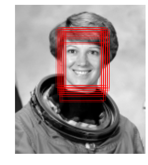
We are detecting the face by using a sliding window which goes over the image patches. Then we find the HOG feature of these patches. Finally, we run it through the classification model that we build and predict the face in the image. The image below is one of the test images. We can see that the classifier detected patches and most of them overlap the face in the image.
To see the full code for this post check out this repository