
Open-Source Internship opportunity by OpenGenus for programmers. Apply now.
Reading time: 45 minutes
Principal Component Analysis (PCA) is a popular dimensionality reduction technique widely used in machine learning. Whitening (or Sphering) is a technique used to reduce redundancy in the input data. Before diving into the concept of whitening, we will first brush up our concepts of PCA. After completing this article, you will have knowledge about the following normalization
- covariance matrix
- eigen vectors and eigen values
- principal components
- how to decide the value of k in PCA
- PCA
- Whitening
PRINCIPAL COMPONENT ANALYSIS (PCA)
When training our model on images, we have a huge number of features. For example, if we are working on a 16 X 16 grayscale image, we will have 256 number of input features. There would be a lot of redundancy here and we might want to reduce the number of input features to, say, 50. PCA would then be the answer to this problem. Let’s take another example where we are training our model to predict the price of a house based on a larger number of input features about the house like area, number of rooms, colour of the rooms, etc. Suppose the number of features is quite large and we are not able to check for each features separately. Now, one feature tells us the area of the house in meter square and another feature tells us the area in feet square. Now both of these are linearly dependent on each other and hence cause redundancy in our input data. We would definitely want to remove one of these features. Again, PCA is the answer.
Working
Let us say, we have n = 256 number of input features and m = 1000 number of training examples (Notice m >> n). Now let us say, we want to reduce the number of features to k = 50 most important features. From these assumptions, we have,
$
x\ :\ n\ X\ m\ matrix\\
x^{(i)}\ :\ i^{th}\ traning\ example\\
x^{(i)}_j\ :\ j^{th}\ training\ feature\ of\ i^{th}\ training\ example\\
x \in \Re^n\\
y\ :\ k\ X\ m\ matrix\ (After\ applying\ PCA\ on\ x)\\
y \in \Re^k\ (new\ data\ points)\
$
Normalization
First, we have to transform our input data in such a way that it has zero mean and unit variance. For that :
$1.\ Let\ \mu\ =\ \frac{1}{m}\sum_{i=1}^mx^{(i)}$
$2.\ Replace\ each\ x^{(i)}\ with\ x^{(i)}\ -\ \mu$
$3.\ Let\ \sigma_{j}^2\ =\ \frac{1}{m}\sum_{i=1}^m(x^{(i)}_{j})^2$
$4.\ Replace\ each\ x^{(i)}_j\ with\ x^{(i)}_j/\sigma _j$
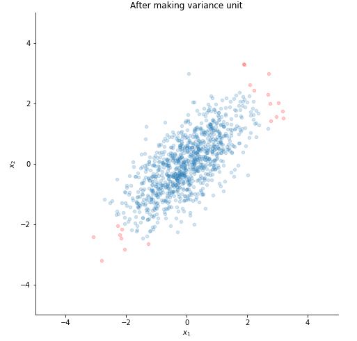
Step 1 and 2 will convert the data to have zero mean and step 3 and 4 will make the variance unit. Unit variance is needed to make sure that all the features are considered on same scale. Suppose one input features can take values between 0 to 1000 and another feature can take only from 0 to 10. Normalisation of data to make their variance unit, will make sure that both these features are treated the same. Such normalization is required in images of handwrtten digits or images of object with white background. It is not required on natural images that is, the images that we see through our eyes for most part of our lives.
FINDING PRINCIPAL COMPONENTS
$x^{(i)}$ is nothing but a point in an n-Dimensional space. If $x^{(i)}$ is the point and a is the projection of this point on a vector v, then the distance of the origin from point a is called the variance of $x^{(i)}$ along v. Now we need to find n such vectors in this n-D space, along which, if these points ($x^{(i)}$) are projected, the projection captures maximum variance. These n vectors are nothing but the Eigen vectors of the covariance matrix ($\Sigma$) of X (assuming we have already applied the zero mean normalization). Eigen vectors are those vectors on which, if we apply any linear transformation (like multiplying by a scalar), its direction doesn't change (For more information, read this article).
$$\Sigma\ =\ \frac{1}{m}\sum_{i=1}^m\ (x^{(i)})(x^{(i)})^T $$
Matrix U contains all the eigen vectors of the cov mat. Each column of matrix U contains 1 eigen vector. These eigen vectors are arranged in the descending order of the eigen value corresponding to each of the eigen vector.
$$U\ =\ \begin{bmatrix} | & | & \ & |\\ u_1 & u_2 & \ldots & u_n\\ | & | & \ & | \end{bmatrix}$$
Note that, higher the eigen value of a eigen vector, higher is the variance captured by it.
We select the eigen vector with highest eigen value and multiply it with a data point $x^{(i)}$.
$y^{(i)}[0]\ =\ u_{1}^T*x^{(i)}$
where $y^{(i)}[0]$ represents the the principal component of $x^{(i)}$
Similarly,
$y^{(i)}[1]\ =\ u_{2}^T*x^{(i)}$
where $y^{(i)}[1]$ represents the the second principal component of $x^{(i)}$
We select top k eigen vectors from matrix U and remove the rest. The new data point which is dimensionally reduced is given by, $y^{(i)}\ =\ U^T*x^{(i)}$
$y^{(i)} \in \Re ^ k$
VALUE OF k
We decide the value of k by fixing the percentage of variance that we want to retain in our data after applying PCA. The percentage of variance is equivalent to the percentage of information that we have retained in our data. For example,we want to retain 99 percent of data (usually we go with 99 percent but this value is application dependent).
We use the following formula:
$$\frac{\sum_{j=1}^k\lambda_j}{\sum_{j=1}^n \lambda_j} \geq 0.99$$
We solve this equation to find the minimum value of k that satisfies the above inequality.
PCA on images
When applying PCA on images, we need to do following normalization as well :
$1. \mu^{(i)} := \frac{1}{n}\sum_{j=1}^{n} x_j^{(i)}$
$2. x_j^{(i)} := x_j^{(i)}\ -\ \mu^{(i)}$
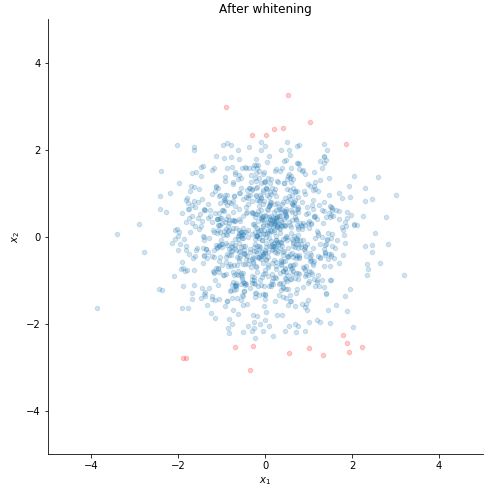
WHITENING
When we are training our model on images, the raw input is quite redundant because the pixels that are adjacent to each other are highly correlated. The goal of Whitening is to reduce redundancy in these images by using 2 measures:
1- making features less correlated to each other
2- making all features have the same variance
The first measure is achieved when we apply PCA on the data. It is because the matrix U is orthogonal. Thus the features in the new data point $y^{(i)}$ have zero covariance and are thus uncorrelated.
The second measure is achieved using the following formula :
$$y^{(i)}_white = y^{(i)}\ ./ \ \sqrt{\lambda}$$
where, ./ represents element-wise division
and \sqrt{\lambda} is a vector consisting of the square root of eigen values corresponding to the top k eigen vectors that we have chosen previously. So,
$$\sqrt{\lambda} =\ \begin{bmatrix} \sqrt{\lambda_1} \\ \sqrt{\lambda_2} \\ \sqrt{\lambda_3} \\ . \\ . \\ \sqrt{\lambda_k} \end{bmatrix}$$
Here, as you can seen in the formula, we divide the product of the eigen vector and the point $x^{(i)}$ by the square root of the corresponding eigen value.
Coding
import numpy as np
import matplotlib.pyplot as plt

np.random.seed(1)
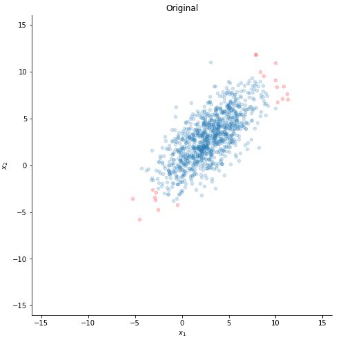
Now let us make our toy dataset. We deliberately take the mean non-zero (here we took mean of each variable as 3) to show you the step making the mean zero. sigma is basically the covariance matrix. As we can see, the covariance between the 2 variables is positive (5 here), so as one variable increases, the other one also increases.
mu = [3,3]
sigma = [[7, 5],[5, 7]] # must be positive semi-definite
n = 1000
x = np.random.multivariate_normal(mu, sigma, size=n).T
Now x is a [2,1000] matrix (2 features and 1000 data points). Now let us choose 20 most extreme points to see how they will change as we operate on the dataset.
set1 = np.argsort(np.linalg.norm(x - 3, axis=0))[-20:]
set2 = list(set(range(n)) - set(set1))
Let us plot our data :D .
def plotting(x, xlim = 16, ylim = 16):
    fig, ax = plt.subplots()
    ax.scatter(x[0, set1], x[1, set1], s=20, c="red", alpha=0.2)
    ax.scatter(x[0, set2], x[1, set2], s=20, alpha=0.2)
    ax.set_aspect("equal")
    ax.set_xlim(-xlim, xlim)
    ax.set_ylim(-ylim, ylim)
    ax.set_xlabel("$x_1$")
    ax.set_ylabel("$x_2$")
    ax.spines["top"].set_visible(False)
    ax.spines["right"].set_visible(False)
    ax.set_title("Original")

plotting(x)
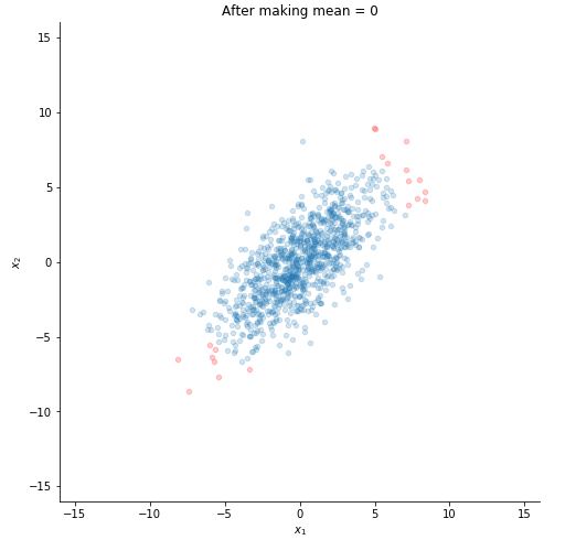
STEP 1 : MAKE THE MEAN ZERO
#m = 1000 here
mu = np.sum(x, axis=1, dtype = np.float32)/1000
for i in range(1000):
    x[:,i] -= mu
Let's plot now to see the difference.
plotting(x, title="After making mean = 0")
STEP 2 : MAKE VARIANCE UNIT
for j in range(x.shape[0]):
    var = np.sum(np.square(x[j,:]), dtype = np.float32)/1000
    for i in range(1000):
        x[j,i] /=  np.sqrt(var)
Plotting it.
STEP 3 : NORMALIZATION IN CASE OF IMAGE DATA (not using here)
'''
n = x.shape[0]

mu = np.sum(x, axis=0,  dtype = np.float32)/n
print (mu.shape)
for i in range(n):
    x[i,:] -=  mu
'''
STEP 4 : FINDING COVARIANCE MATRIX, ITS EIGEN VALUES AND THEIR CORRESPONDING EIGEN VALUES
cov_mat = np.cov(x, rowvar=True)
Lambda, U = np.linalg.eigh(cov_mat)
#Lambda is a 1-D array containing the eigenvalues of cov_mat
#U is a 2D square array of corresponding eigen vectors (in columns)
STEP 5 : DECIDE THE VALUE OF k (not required here as we have only 2 features)
'''
k = 0
percent = 0
s = np.sum(Lambda)
for i in range(Lambda.shape[0]):
    percent = np.sum(Lambda[0:i])/s
    k++
    if (percent >= (a/100)):
        break
    end
'''
For the purpose of illustration let us whiten the data and apply PCA without reducing the number of features.
STEP 6 : WHITEN THE DATA
y = U.T @ x #PCA applied
z = np.diag(Lambda**(-1/2)) @ y #data whitened
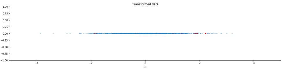
Now let us take k = 1 and plot the new data.
k = 1
y = U[:,0:k].T @ x
z = np.diag(Lambda[0:k]**(-1/2)) @ y

#plotting
y = np.zeros((1,1000))
plt.rcParams['figure.figsize'] = [20, 20]
fig, ax = plt.subplots()
ax.scatter(z[0, set1], y[0, set1], s=20, c="red", alpha=1)
ax.scatter(z[0, set2], y[0, set2], s=20, alpha=0.2)
ax.set_aspect("equal")
ax.set_xlim(-5, 5)
ax.set_ylim(-1, 1)
ax.set_xlabel("$z_1$")
#ax.set_ylabel("$x_2$")
ax.spines["top"].set_visible(False)
ax.spines["right"].set_visible(False)
ax.set_title("Transformed data")
You can also use the function PCA provided by the scikit learn library.
from sklearn.decomposition import PCA
k = 1
pca = PCA(n_components = k, whiten = True)
z = pca.fit_transform(x.T).T

#plotting
y = np.zeros((1,1000))
plt.rcParams['figure.figsize'] = [20, 20]
fig, ax = plt.subplots()
ax.scatter(z[0, set1], y[0, set1], s=20, c="red", alpha=1)
ax.scatter(z[0, set2], y[0, set2], s=20, alpha=0.2)
ax.set_aspect("equal")
ax.set_xlim(-5, 5)
ax.set_ylim(-1, 1)
ax.set_xlabel("$z_1$")
#ax.set_ylabel("$x_2$")
ax.spines["top"].set_visible(False)
ax.spines["right"].set_visible(False)
ax.set_title("Transformed data")
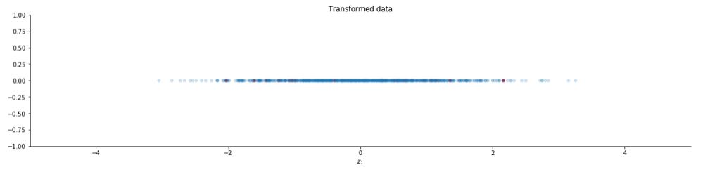
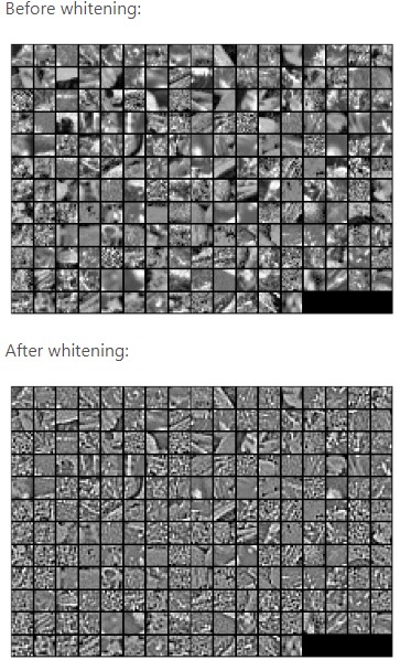
The image is slightly different from the previous one because of slight differences in the PCA function of the scikit learn library. The complete code can be found here. Let us see how whitening looks on images :
Hope you enjoyed the article. Thanks