In this article, we will be exploring a paper titles “Transferability in Machine Learning: from Phenomena to Black-Box Attacks using Adversarial Samples” by Nicolas Papernot, Patric McDaniel and Ian Goodfellow. The paper talks about what adversarial machine learning is and what transferability attacks are. The authors have also presented experimental details on some popular classification systems and have demonstrated adversarial sample transferability. In the end, adversarial crafting techniques are discussed.

Introduction

In this world, there are many fields where machine learning is thriving. Development of technology is taking place at a very fast rate. We can see the application of machine learning algorithms in many places. But it has been proved that machine learning algorithms are vulnerable to adversarial samples. Attacks using such samples basically exploits imperfections and approximations made by learning algorithms.
What is Adversarial sample transferability?
It is the property by which some adversarial sample, that was created to fool or exploit a model is also capable of misleading another model even if the two models have quite different architecture.
In this paper, the authors were able to develop and validate a generalized algorithm for black box attacks that exploit adversarial sample transferability on broad classes of machine learning like DNNs, logistic regression, SVM etc. The contributions of authors in this paper are summarized below:
-The paper shows adversarial sample crafting technique for SVM and decision trees models.
-The paper studies the sample transferability pattern. The models with same ML technique have large sample transfer.
-The paper generalizes the learning of substitute models from deep learning to logistic regression and support vector machines. Another thing shown in the paper is that it is possible to learn substitute matching labels produced by many ML models like DNN, LR etc. at rates superior to 80%.
-The authors conducted attacks against famous classifiers hosted by Amazon and Google. The details can be referred in the paper.

Approach Overview

In this section, we will be discussing the author’s approach towards adversarial sample transferability.
To mislead a model f, solving the following optimization problem will help us get the required adversarial sample:

Here, x(bar) is the proper sample and x(bar)* is the adversarial sample crafted. It is possible that the adversarial sample generated is also misclassified by model f’ which is different from f. Hence, the authors have formalized the adversarial sample transferability notation as follows:

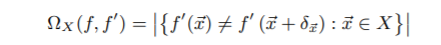
Set X- representative of the expected input distribution for the task solved by model f and f’. Now, the adversarial sample transferability can be partitioned into two variants-

1. Intra-technique transferability- In this, the models f and f’ are trained with same machine learning technique but different parameter initializations or dataset.
2. Cross-technique transferability- Both models f and f’ uses different ML techniques like one is neural network and other is SVM.
   Now, the authors have structured their approach around two hypotheses.
   Hypothesis 1: The above mentioned techniques are both effective and shows/provides significant results.
   In this hypothesis, the authors propose to explore how well the above mentioned two techniques holds for various ML algorithms. This will help us identify the most vulnerable classes of models.
   Hypothesis 2: All unknown machine learning classifiers are vulnerable and prone to black box attacks.
   Note: Validation details including experiment for both hypotheses can be referred in the paper itself.

Transferability of Adversarial Sample in Machine Learning

In this section, we will be briefly discussing the transfer techniques on different machine learning algorithms. For complete experimental details, please refer Section 3 of the paper.
Hypothesis 1 has been used for this study here. The author have explored 5 machine learning algorithms that include DNNs, LR, SVMs, DTs and kNNs. MNIST dataset of handwritten digits has been used for the experimental setup.
For model selection was done using features shown below:

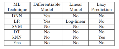
DNNs- for state-of-the-art performance
LR- for its simplicity
SVMs- for their potential robustness
DTs- for their non-differentiability
kNNs- for being lazy-classification models.
Rest of the details can be seen in the paper itself.
Results of experiment

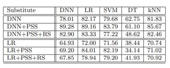
1. It was observed that differentiable models like DNNs and LRs are more vulnerable to intra-technique transferability than non-differentiable models.
2. Another important observation was that LR, SVM, DT and ensembles are vulnerable to cross-technique transferability.

Learning Classifier Substitutes by Knowledge Transfer

To generate or craft samples that are misclassified by a classifier whose details and structure is unknown, substitute model can be used for that. The substitute model solves the same classification problem and its parameters are known.

Dataset Augmentation for Substitutes

Here, the targeted classifier is called oracle as the adversary have the minimal capability of querying it for prediction in inputs of their choice. Only the labels are returned by the oracle. No other details. To overcome this problem, certain data augmentation techniques are used.
Jacobian-based dataset augmentation: This technique is used to learn DNN and LR substitutes. Following steps are involved in this. First, the data is collected. After that, data is labelled by obtaining labels from the oracle. Now, this trained data is used to train the substitute model f. To improve the performance of this model, the following equation is used:

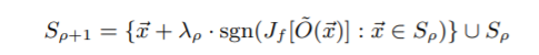
S(p+1): new training set
S(p): previous training set
Lambda(p): a parameter fine-tuning the augmentation step size
J(f): jacobian matrix of substitute
O(x): oracle’s label for sample x
After obtaining the new set S(p+1), the model f is trained using that.
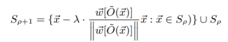
Periodical Step Size: It was shown in the paper that instead of keeping a fixed step size parameter, it will be helpful if the value of this parameter is alternating between positive and negative values. The following equation is used for this:

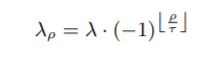
Here, t: number of epochs after which the Jacobian-based dataset augmentation does not lead any improvement.
Reservoir Sampling: To reduce the number of queries made to the oracle, reservoir sampling is used by the author.
The algorithm shown below shows the Jacobian-based augmentation with Reservoir Sampling:

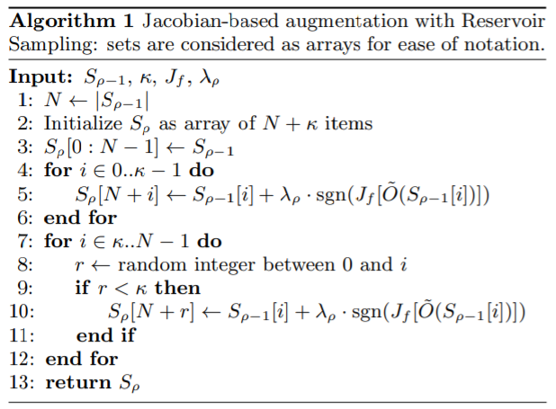
Reservoir sampling chooses k samples randomly from a list of samples. Now as k samples are randomly chosen using reservoir sampling, this will help by avoiding exponential growth of queries made to the oracle when Jacobian-based augmentation is performed.
S(p-1): previous set of substitute training inputs
From this set, k inputs will be augmented to S(p) using reservoir sampling. Each input in S(p-1) will have the probability of 1/|S(p-1)| of being selected. Using this technique, the number of queries is reduced from n.2^p (vanilla Jacobian-based augmentation) to n.2^sigma + k.(p-sigma) (Jacobian-based augmentation with reservoir sampling).

Now let us briefly talk about some machine learning algorithms substitutes. For complete configurations and parameter details, please refer the paper itself.

Deep Neural Network Substitute

The author trained 5 different substitute DNNs to match the labels produced by 5 different oracles, one for each ML technique. MNIST dataset was used. Consider the result plot below:

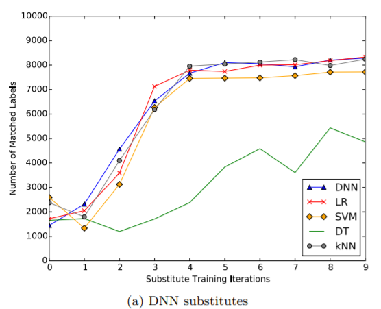
This graph plots at each iteration p the share of samples on which the substitute DNNs agree with predictions made by the classifier oracle they are approximating.

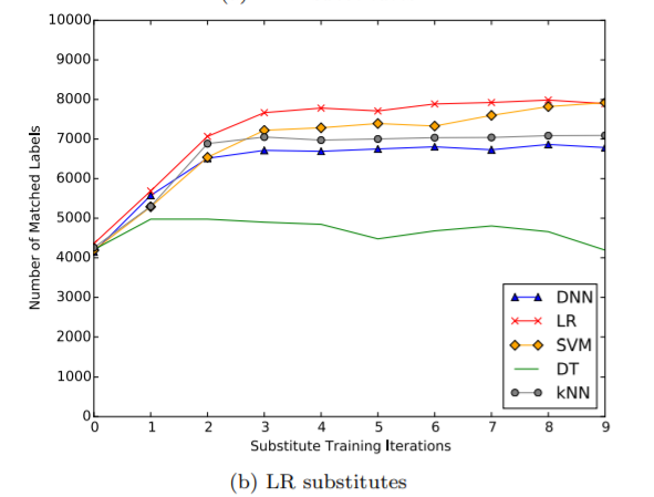
Logistic Regression Substitute

Jacobian-based dataset augmentation is also applicable to multi-class logistic regression. The (i,j) jacobian component of this model can be calculated as follows:

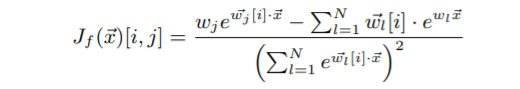
Resultant plot for Logistic regression is shown below:

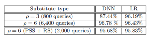
Now, the impact of refinements i.e. Periodic Step Size(PSS) and Reservoir Sampling(RS) on DNN and LR can be summarized in the table below:

Support Vector Machines Substitute

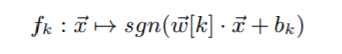
SVM-based dataset augmentation is used to train SVMs to approximate oracles. The following equation is used:

W[k]: weight indicating hyperplane direction of subclassifier k
Note: Please refer the paper for experimental validation of SVM substitute.

Black-Box Attacks of Remote Machine Learning Classifiers

The Oracle Attack Method

The attack method includes locally training a substitute. The authors preferred the use of DNNs and LRs for the substitutes. The two refinements were also applied i.e. Periodical step size and reservoir sampling. The authors targeted two models hosted by Amazon and Google. Step by step details for these attacks are presented in the paper.
1. Amazon Web Services: The model was trained using Amazon machine learning which is provided as a part of Amazon Web Services platform. The table below shows the results obtained:

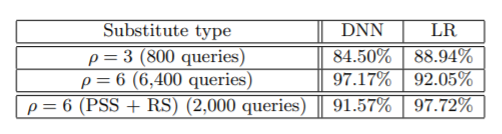
2. Google Cloud Prediction Oracle: The procedure to train model on Google is similar to Amazon. The results obtained are as follows:

Adversarial Sample Crafting

The methods used in the paper for crafting adversarial samples are discussed next:

1. Deep Neural Network: For crafting adversarial sample that are misclassified by NN, the effective method that can be used is fast gradient method given the adversary has the knowledge of model and its parameters. The Jacobian based iterative approach can also be used. In the paper, authors have used fast gradient method.
2. Multi-class Logistic Regression: In multi-class logistic regression, there are more than 2 classes present. The model can be described as:
   
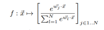
   For this also, fast-gradient sign method is used.
3. Nearest Neighbour: This algorithm is known to be lazy-learning non-parametric classifier. It does not require training phase. In this, k nearest points are considered for classification of unseen points. In this paper, k=1, the model can be shown as:
   
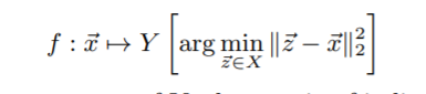
   The authors implemented fast gradient method for generation of adversarial samples. The smoothed version of kNN was used which is given as:
   
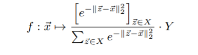
4. Multi-class Support Vector Machines: The equation for this model is given as:
   
   For crafting adversarial sample here, the authors have introduced a method that is computationally efficient and does not require optimization. To craft samples, perturbation of a given input in a direction orthogonal to the decision boundary hyperplane is done. This is shown in the below figure:
   
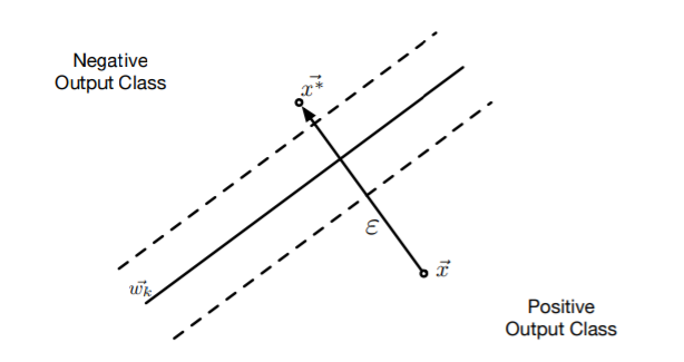
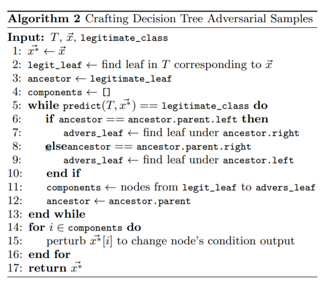
   The figure shows for a binary classifier. For multiclass SVM, the formalized equation can be given as:
   
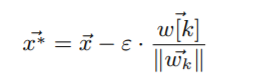
   Here, ||.|| is the Frobenius norm, w[k] is the weight vector. K and e are input variation parameters that controls distortions.
5. Decision trees: For crafting of sample for decision tree, the authors propose to search for leaves with different classes in the neighbourhood of the leaf corresponding to the original prediction. Then find the path from original leaf to the adversarial leaf and modify the sample accordingly to the conditions on this path so as to force the decision tree to misclassify the sample.
   
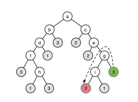
   The below algorithm implements the idea shown in the above figure:
   
   In decision trees, each node has an if-else condition. The trees are traversed and the final leaf reached depicts the final class. All we have to do here for adversarial samples is that modify neighbours of correct class such that the sample is classified to some other class. In the tree structure above, to misclassify sample from class 3 (green leaf), the adversary modifies it such that conditions g and i evaluate such that sample to be classified in class 2 (red leaf). In this algorithm, decision tree T, a sample x(bar) and a legitimate_class for this sample are given as the input and we will assign x(bar)* i.e. the adversarial sample as the normal sample.
   Next, we assign the legit_leaf as the leaf in T corresponding to sample x(bar) and ancestor as the legitimate_leaf.
   Now, we will loop until the sample is misclassified. During this loop, we will modify the neighbours of the correct class. During this loop, we will add nodes from legit_leaf to advers_leaf to component list. Finally, using these components values, we will try to change or alter the node’s condition output.
   Finally, we will return the adversarial sample.

Conclusion

So what we have learnt is that the adversary can even attack models whose model and parameter knowledge is not known. We also saw that, samples crafted for a model f, and even misclassified by model f’, where the sample may or may not be using the same machine learning algorithm. There were also details regarding substitutes that can be used for misclassification. Finally, for different machine learning algorithms crafting methods were explored.