Open-Source Internship opportunity by OpenGenus for programmers. Apply now.
Reading time: 15 minutes
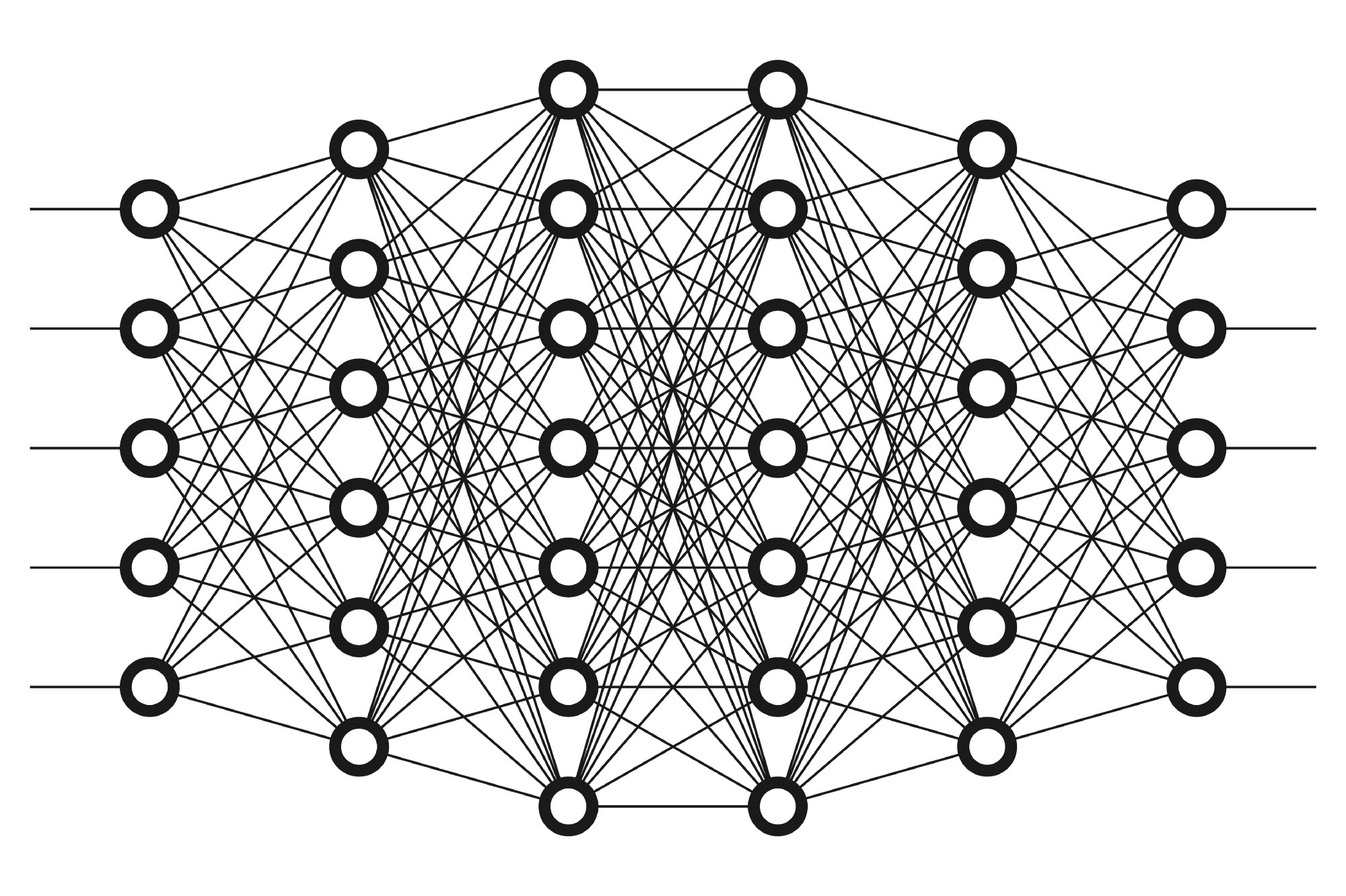
An Artificial Neural Network (henceforth ANN) is a form of computing system that vaguely resembles the biological nervous system. It is composed of very many neurons that are centres of computation and learn by a sort of hit and trial method over the course of many epochs. One can correctly say that an ANN and a perceptron function in an identical fashion. Much rather, the ANN is actually derived from the perceptron to render a more accurate output.

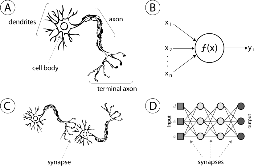
Perceptron versus Artificial Neural Networks
An Artificial Neural Networks is nothing but a multi-layered perceptron structure. Unlike a perceptron, an Artificial Neural Networks most certainly has more than one neuron in the hidden (computation) layer and usually has more than one hidden layers.

From the figure, one can infer that a perceptron is analogous to the functioning of a single neuron in taking in the input and formulating the output. However, when a multitude of such neurons work together to calculate the output whilst transferring the information from layer to layer, the system becomes more functioning and the output is more accurate. This is because of the slightly more sophisticated structure of the neural networks as compared to the perceptron.
Working
Similar to the perceptron, the ANNs take in the values from the input layer and prior to entering the hidden layers, the inputs are weight adjusted i.e. each synapse is assigned a random weight, each input is multiplied by the corresponding weight and all these products are added. After entering the hidden layers, this sum of products is put into an activation function (which could be the tanh or the sigmoid functions for more sophisticated models and simply the Heaviside unit step function for more basic models). This result is tallied with the ground truths and the error generated is minimised through back-propagation.
Stochastic Gradient Descent
For minimising the error or the cost function, we back-propagate the error as followed:
-
Start at a random point on the cost function (which is a function of the predicted output)
-
Find the derivative of the cost function
-
Repeat step 4 until the derivative is equal to 0
-
If the derivative is less than 0, move to the right i.e. the predicted output should be greater than current output, else if the derivative is greater than 0, move to the left i.e. the predicted output should be less than current output.
To prevent ending up at a local minimum of the cost function, one should ideally carry out the back-propagation after every row of the dataset. This process is called the Stochastic Gradient Descent, where stochastic refers to randomly determined processes, alluding to the randomisation of weights and gradient descent essentially means that we are descending through the gradient (slope, derivative) until we reach zero.
Training the ANN
Training of the ANN can be compiled into the following steps:
-
Initialise random weights to values close to 0 (but not 0).
-
Input first row of dataset into the input layer, with each variable assigned to each node of the layer.
-
Forward Propagation: Information flows from left to right. In the neurons, input values are multiplied with their corresponding weights and the products are added, thereafter the activation function acts on this sum of products and renders the output.
-
Compare the rendered output to the actual result and measure the generated error.
-
Back-Propagation: Information flows from right to left. Weights are updated by how much they are responsible for the error and the learning rate decides by how much we update the weights.
-
Repeat steps 1 through 5 and update the weights after each observation (Reinforcement Learning) or update the weights after a batch of observations (Batch Learning).
-
When the whole training set is passed through the ANN, it is called an epoch. Redo more epochs.
Implementations
This is a simple classifier model based on artificial neural networks.
We have added comments to make the code self explainatory. If you have doubts, you can always ask us by commenting in the comment section.
import numpy as np
from sklearn import datasets, linear_model
import matplotlib.pyplot as plt


class Config:
    nn_input_dim = 2  # input layer dimensionality
    nn_output_dim = 2  # output layer dimensionality
    # Gradient descent parameters
    epsilon = 0.01  # learning rate for gradient descent
    reg_lambda = 0.01  # regularization strength


def generate_data():
    np.random.seed(0)
    X, y = datasets.make_moons(200, noise=0.20)
    return X, y


def visualize(X, y, model):
    # plt.scatter(X[:, 0], X[:, 1], s=40, c=y, cmap=plt.cm.Spectral)
    # plt.show()
    plot_decision_boundary(lambda x:predict(model,x), X, y)
    plt.title("Logistic Regression")


def plot_decision_boundary(pred_func, X, y):
    # Set min and max values and give it some padding
    x_min, x_max = X[:, 0].min() - .5, X[:, 0].max() + .5
    y_min, y_max = X[:, 1].min() - .5, X[:, 1].max() + .5
    h = 0.01
    # Generate a grid of points with distance h between them
    xx, yy = np.meshgrid(np.arange(x_min, x_max, h), np.arange(y_min, y_max, h))
    # Predict the function value for the whole gid
    Z = pred_func(np.c_[xx.ravel(), yy.ravel()])
    Z = Z.reshape(xx.shape)
    # Plot the contour and training examples
    plt.contourf(xx, yy, Z, cmap=plt.cm.Spectral)
    plt.scatter(X[:, 0], X[:, 1], c=y, cmap=plt.cm.Spectral)
    plt.show()


# Helper function to evaluate the total loss on the dataset
def calculate_loss(model, X, y):
    num_examples = len(X)  # training set size
    W1, b1, W2, b2 = model['W1'], model['b1'], model['W2'], model['b2']
    # Forward propagation to calculate our predictions
    z1 = X.dot(W1) + b1
    a1 = np.tanh(z1)
    z2 = a1.dot(W2) + b2
    exp_scores = np.exp(z2)
    probs = exp_scores / np.sum(exp_scores, axis=1, keepdims=True)
    # Calculating the loss
    corect_logprobs = -np.log(probs[range(num_examples), y])
    data_loss = np.sum(corect_logprobs)
    # Add regulatization term to loss (optional)
    data_loss += Config.reg_lambda / 2 * (np.sum(np.square(W1)) + np.sum(np.square(W2)))
    return 1. / num_examples * data_loss


def predict(model, x):
    W1, b1, W2, b2 = model['W1'], model['b1'], model['W2'], model['b2']
    # Forward propagation
    z1 = x.dot(W1) + b1
    a1 = np.tanh(z1)
    z2 = a1.dot(W2) + b2
    exp_scores = np.exp(z2)
    probs = exp_scores / np.sum(exp_scores, axis=1, keepdims=True)
    return np.argmax(probs, axis=1)


def build_model(X, y, nn_hdim, num_passes=20000, print_loss=False):
    # Initialize the parameters to random values. We need to learn these.
    num_examples = len(X)
    np.random.seed(0)
    W1 = np.random.randn(Config.nn_input_dim, nn_hdim) / np.sqrt(Config.nn_input_dim)
    b1 = np.zeros((1, nn_hdim))
    W2 = np.random.randn(nn_hdim, Config.nn_output_dim) / np.sqrt(nn_hdim)
    b2 = np.zeros((1, Config.nn_output_dim))

    # This is what we return at the end
    model = {}

    # Gradient descent. For each batch...
    for i in range(0, num_passes):

        # Forward propagation
        z1 = X.dot(W1) + b1
        a1 = np.tanh(z1)
        z2 = a1.dot(W2) + b2
        exp_scores = np.exp(z2)
        probs = exp_scores / np.sum(exp_scores, axis=1, keepdims=True)

        # Backpropagation
        delta3 = probs
        delta3[range(num_examples), y] -= 1
        dW2 = (a1.T).dot(delta3)
        db2 = np.sum(delta3, axis=0, keepdims=True)
        delta2 = delta3.dot(W2.T) * (1 - np.power(a1, 2))
        dW1 = np.dot(X.T, delta2)
        db1 = np.sum(delta2, axis=0)

        # Add regularization terms (b1 and b2 don't have regularization terms)
        dW2 += Config.reg_lambda * W2
        dW1 += Config.reg_lambda * W1

        # Gradient descent parameter update
        W1 += -Config.epsilon * dW1
        b1 += -Config.epsilon * db1
        W2 += -Config.epsilon * dW2
        b2 += -Config.epsilon * db2

        # Assign new parameters to the model
        model = {'W1': W1, 'b1': b1, 'W2': W2, 'b2': b2}

        # Optionally print the loss.
        # This is expensive because it uses the whole dataset, so we don't want to do it too often.
        if print_loss and i % 1000 == 0:
            print("Loss after iteration %i: %f" % (i, calculate_loss(model, X, y)))

    return model


def classify(X, y):
    # clf = linear_model.LogisticRegressionCV()
    # clf.fit(X, y)
    # return clf

    pass


def main():
    X, y = generate_data()
    model = build_model(X, y, 3, print_loss=True)
    visualize(X, y, model)


if __name__ == "__main__":
    main()
Output
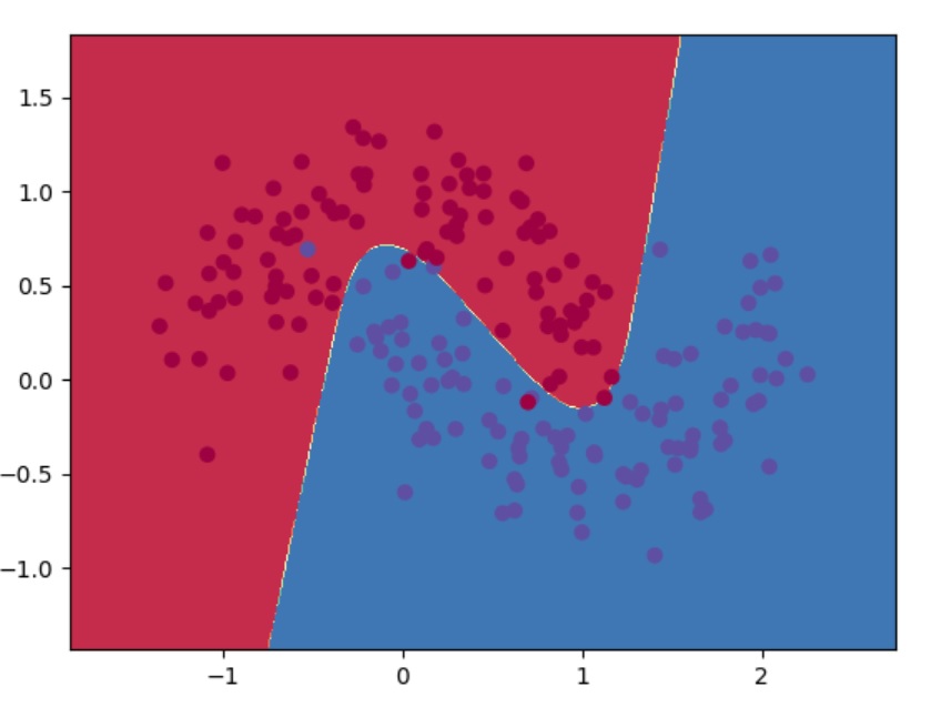
This is the final classification output of the above code:

As you can see from the output that the loss is decreasing with each iteration and has reached a local minima after 13000 iterations.
Loss after iteration 0: 0.432387
Loss after iteration 1000: 0.068947
Loss after iteration 2000: 0.068936
Loss after iteration 3000: 0.071218
Loss after iteration 4000: 0.071253
Loss after iteration 5000: 0.071278
Loss after iteration 6000: 0.071293
Loss after iteration 7000: 0.071303
Loss after iteration 8000: 0.071308
Loss after iteration 9000: 0.071312
Loss after iteration 10000: 0.071314
Loss after iteration 11000: 0.071315
Loss after iteration 12000: 0.071315
Loss after iteration 13000: 0.071316
Loss after iteration 14000: 0.071316
Loss after iteration 15000: 0.071316
Loss after iteration 16000: 0.071316
Loss after iteration 17000: 0.071316
Loss after iteration 18000: 0.071316
Loss after iteration 19000: 0.071316
