Open-Source Internship opportunity by OpenGenus for programmers. Apply now.
Reading time: 20 minutes
A Bayesian model is a statistical model where we use probability to represent all uncertainty within the model, both the uncertainty regarding the output but also the uncertainty regarding the input to the model.
The basic idea in a Bayesian model is that we start by assuming something about whatever we are investigating. This is called the prior distribution. Then we adjust that based on our data.
We will understand Bayesian model by exploring Bayesian Linear Regression which is a modification of the Linear regression model using the Bayesian principles.
Bayesian Linear Regression:
Bayesian linear regression is an approach to linear regression in which the statistical analysis is undertaken within the context of Bayesian inference. When the regression model has errors that have a normal distribution, and if a particular form of prior distribution is assumed, explicit results are available for the posterior probability distributions of the model's parameters.
Difference between normal linear regression and bayesian Linear Regression
Normal linear regression is a frequentist approach, and it assumes that there are enough measurements to say something meaningful.
In the Bayesian approach, the data are supplemented with additional information in the form of a prior probability distribution. The prior belief about the parameters is combined with the data's likelihood function according to Bayes theorem to yield the posterior belief about the parameters.
Why Bayesian version?
- Bayesian hierarchical models are easy to extend to many levels
- Bayesian model selection probably superior (BIC/AIC)
- Bayesian models are more flexible so it can handle more complex models
- Bayesian analysis are more accurate in small samples
- Bayesian models can incorporate prior information
Bayesian Inference
Let us understand this with the help of an example suppose:
there is a company that makes biased coins i.e. they adjust the weight of the coins in such a way that the one side of the coin is more likely than the other while tossing. For now let's assume that they make just two types of coins. ‘Coin 1’ with 30% chances to get heads and ‘Coin 2’ with 70% chances to get heads. Now, we have got a coin from this factory and want to know if it is ‘Coin 1’ or ‘Coin 2’. We have been also given that the company makes both the coins in same quantity. This will help us define our prior probability for the problem that is our coin is equally likely to be either ‘Coin 1’ or ‘Coin 2’ or 50-50 chance.
After assigning prior probability, we have tossed the coin 3 times and got heads in all three trials. The Frequentist approach will ask us to take more samples since we cannot accept or refuse the null hypothesis with this sample size at 95% confidence interval. However, as we will see with Bayesian approach each packet of information or trial will modify the prior probability or our belief for the coin to be ‘Coin 2’.
At this point we know the original priors for the coins i.e
P(Coin1)=P(Coin2)=0.5(50%)
Additionally we also know the conditional probability i.e. chances of heads for Coin 1 and Coin 2
P(Heads|Coin1)= 30%
P(Heads|Coin2)= 70%
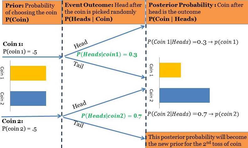
Now we have performed our first experiment or trial and got heads. This is a new information for us and this will help calculate the posterior probability of coins when heads has happened.

If we insert the values to the above formula the chances for Coin1 have gone down

Similarly chances for Coin 2 have gone up

This same experiment is shown in the figure below:

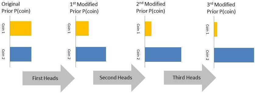
As mentioned in the above figure the posterior probabilities of the first toss i.e. P(Coin 1|Heads) and P(Coin 2|Heads) will become the prior probabilities for the subsequent experiment. In the next two experiments we have further got 2 more heads this will further modify the priors for the fourth experiment as shown below. Each packet of information is improving your belief about the coin as shown below:

By the end of the 3rd experiment we are almost 90% sure that we have a coin that resembles Coin 2. The above example is a special case since we have considered just two coins. However, for most practical problems we will have factories that produce coins of all different biases. In such cases the prior probabilities will be a continuous distribution.
Summary
In this article we learned about Bayesian model and bayesian linear regression. We also studied that why do we go for bayesian version instead of normal one.At the end we studied in detail about bayesian inference.
In next article we will study about Naive Bayes theorem.
