
Open-Source Internship opportunity by OpenGenus for programmers. Apply now.
Reading time: 35 minutes | Coding time: 10 minutes
As the title sugests, Root-Finding Problem is the problem of finding a root of an equation f(x) = 0, where f(x) is a function of a single variable x. The problem is stated as follows:
Given a continuous function f(x).
Find a number x = c such that f(c) = 0.
The root-finding problem is one of the most important computational problems. It arises in a wide variety of practical applications in physics, chemistry, biosciences, engineering, etc.
Why use Numerical Methods for Root Finding Problems ?
Except for some very special functions, it is not possible to find an analytical expression for the root, from where the solution can be exactly determined.
You may have learned how to solve a quadratic equation :

Unfortunately, such analytical formulas do not exist for polynomials of degree 5 or greater as stated by Abel–Ruffini theorem.
Thus, most computational methods for the root-finding problem have to be iterative in nature. The main idea is to first take an initial approximation of the root and produce a sequence of numbers (each iteration providing more accurate approximation to the root in an ideal case) that will converge towards the root. Since the iteration must be stopped at some point these methods produce an approximation to the root, not an exact solution.
In this post we wil explore:
- Bisection Method
Bisection Method
Theory
The Bisection Method, also called the interval halving method, the binary search method, or the dichotomy method is based on the Bolzano’s theorem for continuous functions (corollary of Intermediate value theorem).
Theorem (Bolzano) : If the function f(x) is continuous in [a, b] and f(a)f(b) < 0 (i.e. f(x) has opposite signs signs at a and b)
then a value c ∈ (a, b) exists such that f(c) = 0.
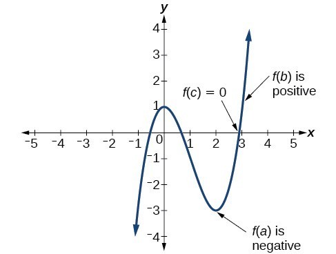
The Bisection Method looks to find the value c for which the plot of the function f crosses the x-axis. The c value is in this case is an approximation of the root of the function f(x). How close the value of c gets to the real root depends on the value of the tolerance we set for the algorithm.
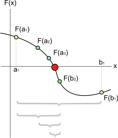
Image Source : https://en.wikipedia.org/wiki/File:Bisection_method.png
Algorithm
For a given function f(x),the Bisection Method algorithm works as follows:
1. Start

2. Define function f(x)

3. Input
	a. Lower and Upper guesses a and b
	b. tolerable error e

4. If f(a)*f(b) > 0
	print "Incorrect initial guesses"
   	goto 3
   End If

5. Do
	c = (a+b)/2

	If f(a)*f(c) < 0
		b = c
	Else
		a = c
	End If

   while (fabs(f(c)) > e)   // fabs -> returns absolute value

6. Print root as c

7. Stop
Sample Problem
Now let's work with an example:
Show that f(x) = x3 + 4x2 - 10 has a root in [1,2], and use the Bisection method to determine an approximation to the root that is accurate to at least within 10-6.
Now, the information required to perform the Bisection Method is as follow:
- f(x) = x3 + 4x2 - 10,
- Lower Guess a = 1,
- Upper Guess b = 2,
- And tolerance e = 10-6
We know that f(a) = f(1) = -5 (negative) and f(b) = f(2) = 14 (positive) so the Intermediate Value Theorem ensures that the root of the function f(x) lies in the interval [1,2].
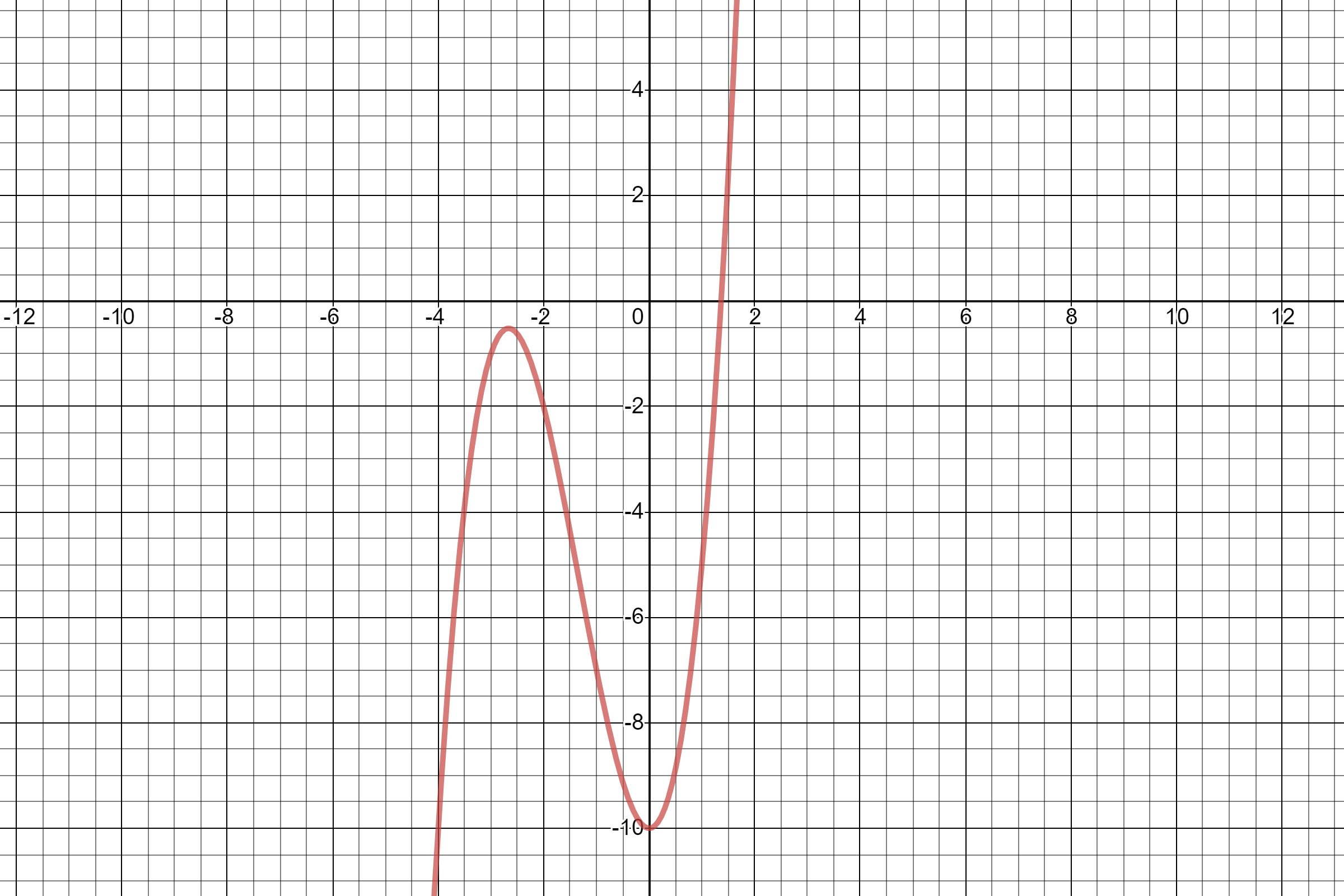
Below we show the iterative process described in the algortihm above and show the values in each iteration:
- Inputs
- f(x) = x3 + 4x2 - 10,
- Lower Guess a = 1,
- Upper Guess b = 2,
- And tolerance e = 10-6
Iteration 1
a = 1, b = 2
-
Check if f(a) and f(b) have opposite signs
f(a) = f(1) = -5 ; f(b) = f(2) = 14
So, f(a)*f(b) = f(1)*f(2) = -70 < 0 ✅ -
We then proceed to calculate c :
c = (a+b)/2 = (1+2)/2 = 1.5
c=1.5 -
Check if f(a) and f(c) have opposite signs
f(a) = f(1) = -5 ; f(c) = f(1.5) = 2.375
f(a)*f(c) = f(1)*f(1.5) = -11.875 < 0 ✅
Since the above condition is satisfied, we make c as our new upper guess i.e. b
b = c
b = 1.5
So, we have reduced the interval to half of the original.
[1,2] -> [1,1.5] -
Now we check the loop condition i.e. fabs(f(c)) > e
f(c) = 2.375
fabs(f(c)) = 2.375 > e = 10-6 ✅
The loop condition is true so we will perform the next iteration.
Iteration 2
a = 1, b = 1.5
-
Check if f(a) and f(b) have opposite signs
f(a) = f(1) = -5 ; f(b) = f(1.5) = 2.375
So, f(a)*f(b) = f(1)*f(1.5) = -11.875 < 0 ✅ -
We then proceed to calculate c :
c = (a+b)/2 = (1+1.5)/2 = 1.25
c=1.25 -
Check if f(a) and f(c) have opposite signs
f(a) = f(1) = -5 ; f(c) = f(1.25) = -1.796875
f(a)*f(c) = f(1)*f(1.25) = 8.984375 < 0 ❌
Since the above condition is not satisfied, we make c as our new lower guess i.e. a
a = c
a = 1.25
Again we have reduced the interval to half of the original.
[1,1.5] -> [1.25,1.5] -
Now we check the loop condition i.e. fabs(f(c)) > e
f(c) = -1.796875
fabs(f(c)) = 1.79685 > e = 10-6 ✅
The loop condition is true so we will perform the next iteration.
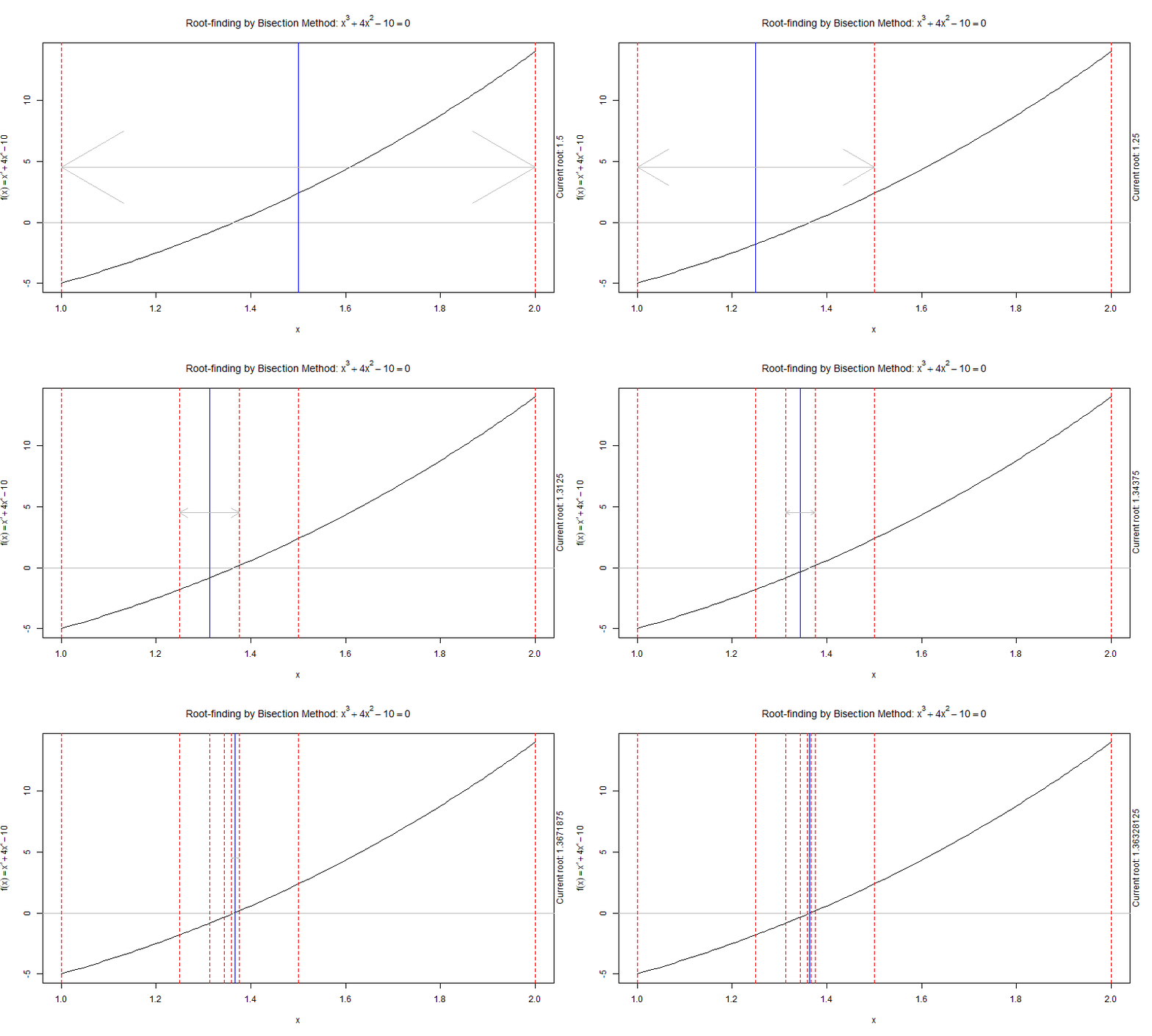
As you can see, the Bisection Method converges to a solution which depends on the tolerance and number of iteration the algorithm performs.
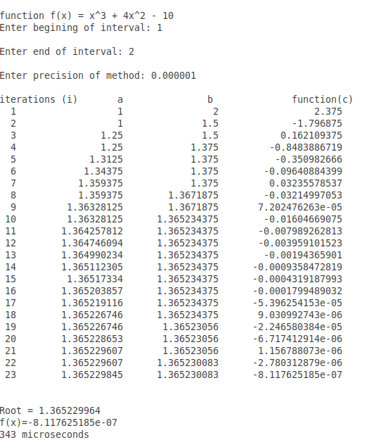
C++ Implementation
#include <iostream>
#include <math.h>
#include<iomanip>
#include<chrono>
using namespace std::chrono;
using namespace std;


static double function(double x); // function f(x)
void menu();


int main() {

  double a; // Lower Guess or beginning of interval
  double b; // Upper Guess or end of interval
  double c; // variable for midpoint
  double precision;

  cout << "\n\n\nfunction f(x) = x^3 + 4x^2 - 10  "<<endl;

  // Taking Input
  cout << "Enter begining of interval: ";
  cin >> a;
  cout << "\nEnter end of interval: ";
  cin >> b;
  cout << "\nEnter precision of method: ";
  cin >> precision;

  // Check for opposite sign (Intermediate Value Theorem)
  if (function(a) * function(b) > 0.0f)
  {
    cout << "\nFunction has same signs at ends of interval";
    return -1;
  }

int iter=0;
cout<<setw(3)<<"\niterations (i)"<<setw(8)<<"a"<<setw(16)<<"b"<<setw(25)<<"function(c)"<<endl;

auto start = high_resolution_clock::now();

  do
  {
    c = (a + b) / 2.0f;

    iter++;
    cout<<setprecision(10)<<setw(3)<<iter<<setw(19)<<a<<setw(17)<<b<<setw(22)<<function(c)<<endl;

    // check for opposite sign
    if (function(a) * function(c) < 0.0f)
    {
      b = c;
    }
    else
    {
      a = c;
    }
  }while (fabs(function(c))>=precision);  // terminating condition

  auto stop = high_resolution_clock::now();
  auto duration = duration_cast<microseconds>(stop - start);

  cout<<"\n\nRoot = "<<c<<endl;
  cout<<"f(x)="<<function(c)<<endl;
  cout << duration.count()<<" microseconds"<< endl;

  return 0;
}

static double function(double x)
{
  return pow(x,3) + 4*pow(x,2) - 10 ;
}
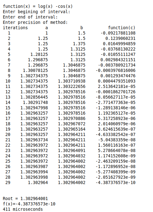
Another Example
Limitations
While Bisection Method is always convergent, meaning that it is always leading towards a definite limit and relatively simple to understand there are some drawbacks when this algorithm is used.
-
Slow rate of convergence
The convergence of the bisection method is slow as it is simply based on halving the interval. -
Relies on sign changes
If a function f (x) is such that it just touches the x -axis for example say f(x) = x2 then it will not be able to find lower guess (a) such that f(a)*f(b) < 0 -
Cannot detect Multiple Roots
The Bisection method fails to identify multiple different roots, which makes it less desirable to use compared to other methods that can identify multiple roots. When an equation has multiple roots, it is the choice of the initial interval provided by the user which determines which root is located.
