
Get this book -> Problems on Array: For Interviews and Competitive Programming
Key takeaways of this research:
- By assuming indexes are models, all index structures can be replaced with other types of models (“learned indexes”)
- Models can learn the sort order or structure of lookup keys – this can be used to predict the position or existence of records
- Using neural nets and learned indexes, cache-optimised B-Trees can be outperformed by up to 70% in speed, while saving an order-of-magnitude in memory
- Replacement of core components of a data management system with learned models will have an impact on future systems designs
Outline
- This paper outlines and evaluates the potential of a new approach to build indexes – this complements existing work but opens up a new research direction in an established field
- The same semantic guarantees can be provided by decomposing data structures into a learned model and auxiliary structure
- Continuous functions describing data distribution can be used to build more efficient data structures or algorithms
- The concept of learned indexes will be introduced by using B-Trees as a model, then Hash-maps and Bloom Filters
- Conclusion: Learned indexes outperform traditional index structures
Main Challenges facing the design of learned index structures
- Index structures are used for efficient data requests and are made to be more energy/cache/CPU efficient
o B-Trees: for range requests, i.e. to look up all records in a certain time frame
o Hash-maps: perform well in single-key look ups
o Bloom filters: check for record existence - Indices are general purpose data structures - they do not assume anything about data distribution, and do not take advantage of common patterns prevalent in real-world data – hence giving the opportunity for learned indexes to be a specialized solution to a case
Examining different indices
Range index
Assumptions: only an in-memory dense array that is sorted by key is indexed
Justification: optimized B-Trees, e.g., FAST, make exactly the same assumptions; these indexes are common for in-memory database systems for their superior performance compared to scanning/binary search
Range index structure
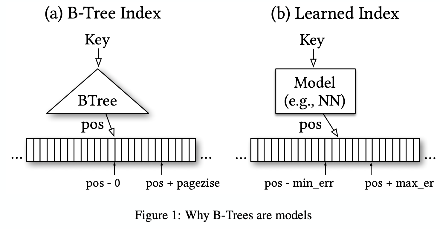
- Already models (similar to B-Trees)
- Given a key, they “predict” the location of a value within a key-sorted set
- Only the key of every n-th record, i.e., the first key of a page, is indexed – this is done for efficiency reasons, reduces the number of keys the index has to store without affecting performance
- Assume fixed-length records and logical paging over a continuous memory region, i.e., a single array
- B-Tree is a model (regression tree): it maps a key to a position with a min- and max-error (a min-error of 0 and a max-error of the page-size), and a guarantee that the key can be found in that region if it exists
Other types of ML models (incl. neural nets) can replace the learned index as long as they are also able to provide similar strong guarantees about the min- and max-error.
- B-Tree provides the strong min- and max-error guarantee over the stored keys, not for all possible keys (B-Trees need to be re-balanced/re-trained when there is new data to provide the same error guarantees)
- For monotonic models the model has to be executed for every key and the worst over- and under-prediction of a position must be recordedto calculate the min- and max-error
- Strong error bounds are unneeded: Data has to be sorted anyway to support range requests, so any error is easily corrected by a local search around the prediction (e.g., using exponential search) and thus, even allows for non-monotonic models.
Conclusion: B-Trees can be replsced with any other type of regression model, including linear regression or neural nets
Technical Challenges in replacing B-Trees with models
- B-Trees have a bounded cost for inserts and look-ups and use the cache well
- B-Trees can map keys to pages which are not continuously mapped to memory or disk
Benefits of replacing B-Trees with models
- Can transform the log n cost of a B-Tree look-up into a constant operation
o E.g. There is a dataset with 1M unique keys with a value from 1M and 2M (so the value 1,000,009 is stored at position 10).
o A simple linear model (consisting of a single multiplication and addition) can perfectly predict the position of any key for a point look-up or range scan, whereas a B-Tree would require log n operations. - Machine learning, especially neural nets, can learn a wide variety of data distributions, mixtures and other data peculiarities and patterns.
Challenge: balance the complexity of the model with its accuracy.
- Number of operations can be performed in the same amount of time it takes to traverse a B-Tree
- Precision the model needs to achieve to be more efficient than a B-Tree
- Use of machine learning accelerators to run much more complex models in the same amount of time and offload computation from the CPU
Similarity to a CDF
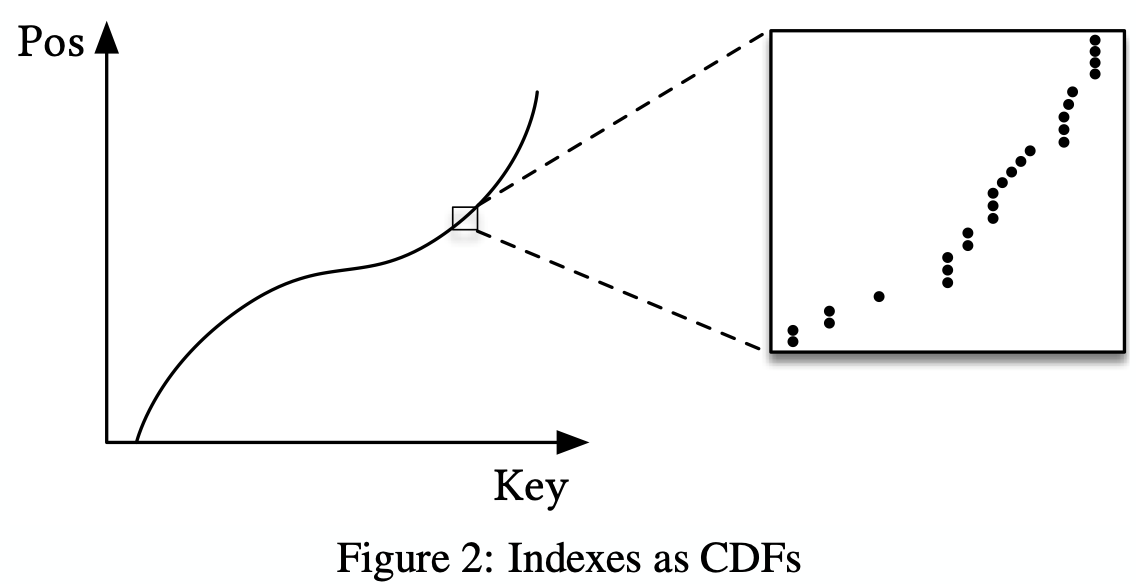
Model that predicts the position given a key inside a sorted array effectively approximates the cumulative distribution function (CDF)
Position can be predicted by p = F (Key) ∗ N
- p is the position estimate
- F (Key) is the estimated cumulative distribution function for the data to estimate the likelihood to observe a key smaller or equal to the look-up key P (X ≤ Key
- N is the total number of keys
Implications
- Indexing requires learning a data distribution
o E.g. B-Tree “learns” the data distribution by building a regression tree;
o E.g.2 Linear regression model would learn the data distribution by minimizing the (squared) error of a linear function - Precedent research is available on estimating the distribution for a dataset
- Learning the CDF plays can help optimize other types of index structures and potential algorithms
- Theoretical CDFs closely approximate empirical CDFs, previous research can help theoretically understand the benefits of this approach
Rough Execution
The look-up time for a randomly selected key (averaged over several runs disregarding the first numbers) was measured with Tensorflow and Python as the front-end
Results:
Tensorflow
≈ 1250 predictions per second
≈ 80, 000 nano-seconds (ns) to execute the model with Tensorflow, without the search time (the time to find the actual record from the predicted position)
B-Tree
traversal over the same data takes ≈ 300ns
binary search over the entire data roughly ≈ 900ns
Challenges with this method:
- Tensorflow designed for larger models, hence it has a large invocation overhead
- B-Trees can quickly overfit the data with a few if-statements, wherease other models are better at approximating the CDF and have problems at the individual data instance level
- B-Trees are extremely cache- and operation-efficient, compared to neural networks which require all weights to compute a prediction (high cost in number of multiplications)
RM Index
Simple, fully-connected neural nets have been used to develop the learning index framework, recursive-model indexes (RMI), and standard-error-based search strategies
Learning index framework
- Index synthesis system; given an index specification, LIF generates different index configurations, optimizes them, and tests them automatically
- Simple models can be learnt on-the-fly (e.g., linear regression models), but Tensorflow is used for more complex models (e.g., NN)
- Staged models can be considered as such
- Inefficiencies: Not instrumentalized to quickly evaluate different index configurations leading to additional overhead in form of additional counters, virtual function calls, etc; Special SIMD intrinisics were not made use of
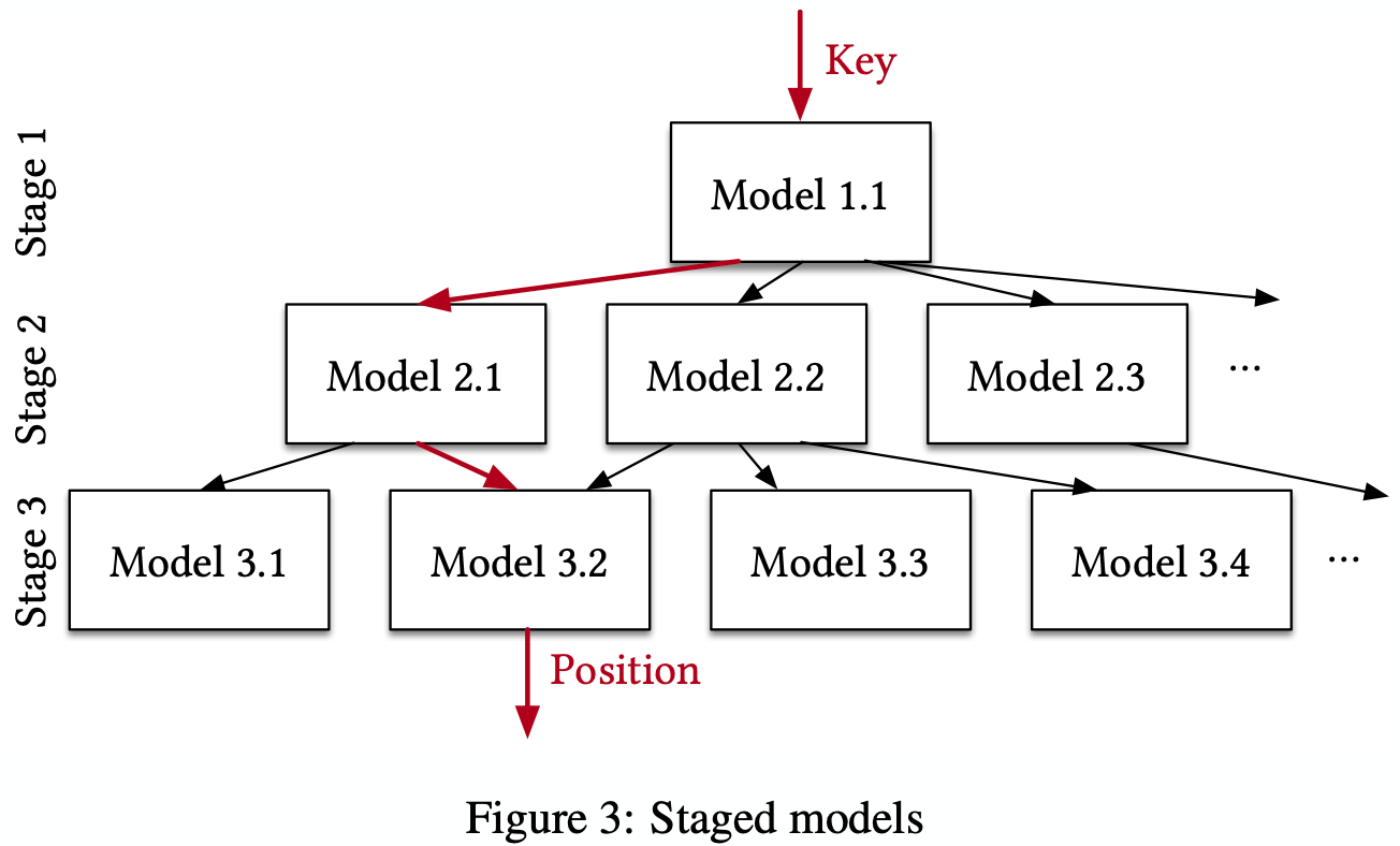
Recursive Model Index
- Tackles the difficulty for accuracy in the last-mile search
- Model:
o For our model f (x) (where x is the key and y ∈ [0, N ) the position], assume at stage l there are M(l) models
o Train the model at stage 0, f0(x) ≈ y
o Model k in stage l, denoted by f (k)(l) is as follows
o f(l-1)(x) recursively executing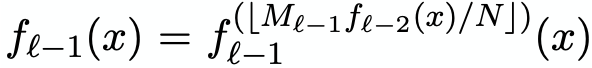
o Iteratively train each stage with f(l-1)(x) for the whole model - Benefits: (1) Separates model size and complexity from execution cost (2) Leverages the fact that it is easy to learn the overall shape of the data distribution (3) Effectively divides the space into smaller sub-ranges like a B-Tree, making it easier to achieve the required “last mile” accuracy with fewer operations (4) No search process required in-between the stages, reducing the number of instructions to manage the structure and the entire index can be represented as a sparse matrix-multiplication for a TPU/GPU.
Algorithm 1: Hybrid End-To-End Training
Input: int threshold, int stages[], NN complexity
Data: record data[], Model index[][]
Result: trained index
1 M = stages.size;
2 tmp records[][];
3 tmp records[1][1] = all data;
4 for i ← 1 to M do
5 	for j ← 1 to stages[i] do
6 		index[i][j] = new NN trained on tmp records[i][j];
7 		if i < M then
8 			for r ∈ tmp records[i][j] do
9 			p = index[i][j](r.key) / stages[i + 1];
10 			tmp records[i + 1][p].add(r);
11 for j ← 1 to index[M ].siz e do
12 	index[M ][j].calc err(tmp records[M ][j]);
13 	if index[M ][j].max abs err > threshold then
14 		index[M ][j] = new B-Tree trained on tmp records[M ][j];
15 return index;
Hybrid index
- Retains benefits of the recursive model index
- The top-node model is first trained starting from the entire dataset (line 3), this prediction helps it pick the model from the next stage (lines 9 and 10) and adds all keys which fall into that model (line 10) then, the index is optimized by replacing NN models with B-Trees if absolute min-/max-error is above a predefined threshold (lines 11-14)
- Hybrid indexes allow us to bound the worst case performance of learned indexes to the performance of B-Trees
Search strategies from learned indexes:
Models actually predict the position of the key, not just the region (i.e., page) of the key
- Model Biased Search: Default search strategy, similar to binary search but the first middle point is set to the value predicted by the model
- Biased Quaternary Search: Quaternary search takes instead of one split point three points with the hope that the hardware pre-fetches all three data points at once to achieve better performance if the data is not in cache. In our implementation, we defined the initial three middle points of quaternary search as pos σ, pos, pos + σ. I.e. assume most of our predictions are accurate and focus our attention first around the position estimate, then we continue with traditional quaternary search
Indexing strings and training
- Turn strings into features for the model (tokenization); Consider an n-length string to be a feature vector x ∈ R^n where x_i is the ASCII decimal value/Unicode decimal value
- Set a maximum input length N because ML operates more efficiently if all inputs are of equal size
- Training is relatively fast by using stochastic gradient descent for simple NNs or closed form solution exists for linear multi-variate models
Results
- Integer Datasets: used data from 2 real-world datasets, (1) Weblogs and (2) Maps, and (3) asynthetic dataset, Lognorma
the main results are as follows
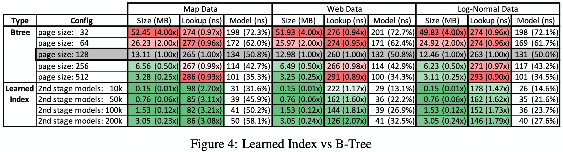
- The learned index was compared with other alternative baselines, including a histogram, lookup-table, FAST, fixed-size B-Tree & interpolation search and learned indexes without overhead
the main results are as follows
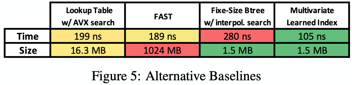
Learned indexes provide the best overall performance while saving significant amount of memory (the FAST index is big because of the alignment requirement) - String Datasets: secondary index was created over 10M non-continuous document-ids of a large web index used as part of a real product at Google
the main results are as shown
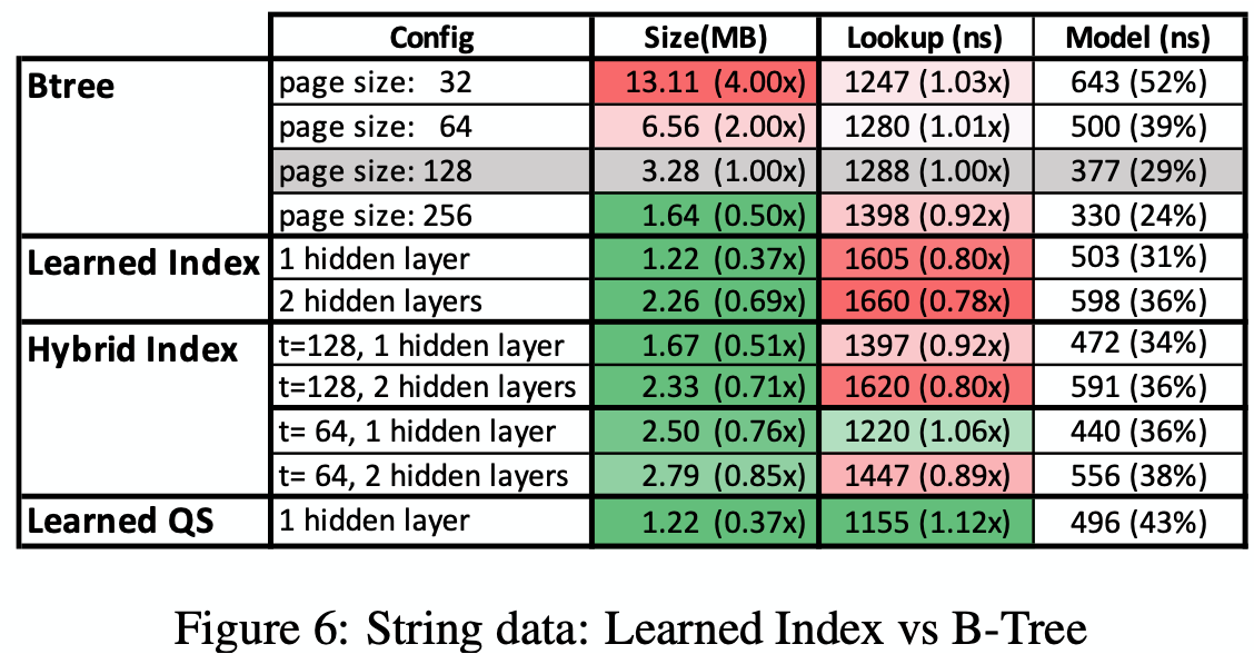
Speedups for learned indexes over B-Trees for strings less obvious, because of the comparably high cost of model execution, a problem that GPU/TPUs would remove; searching over strings is much more expensive thus higher precision often pays off (the reason that hybrid indexes, which replace bad performing models through B-Trees, help to improve performance)
Point Index
- Hash-maps for point look-ups play a similarly important role in DBMS
- Hash-maps use a hash-function to deterministically map keys to positions inside an array
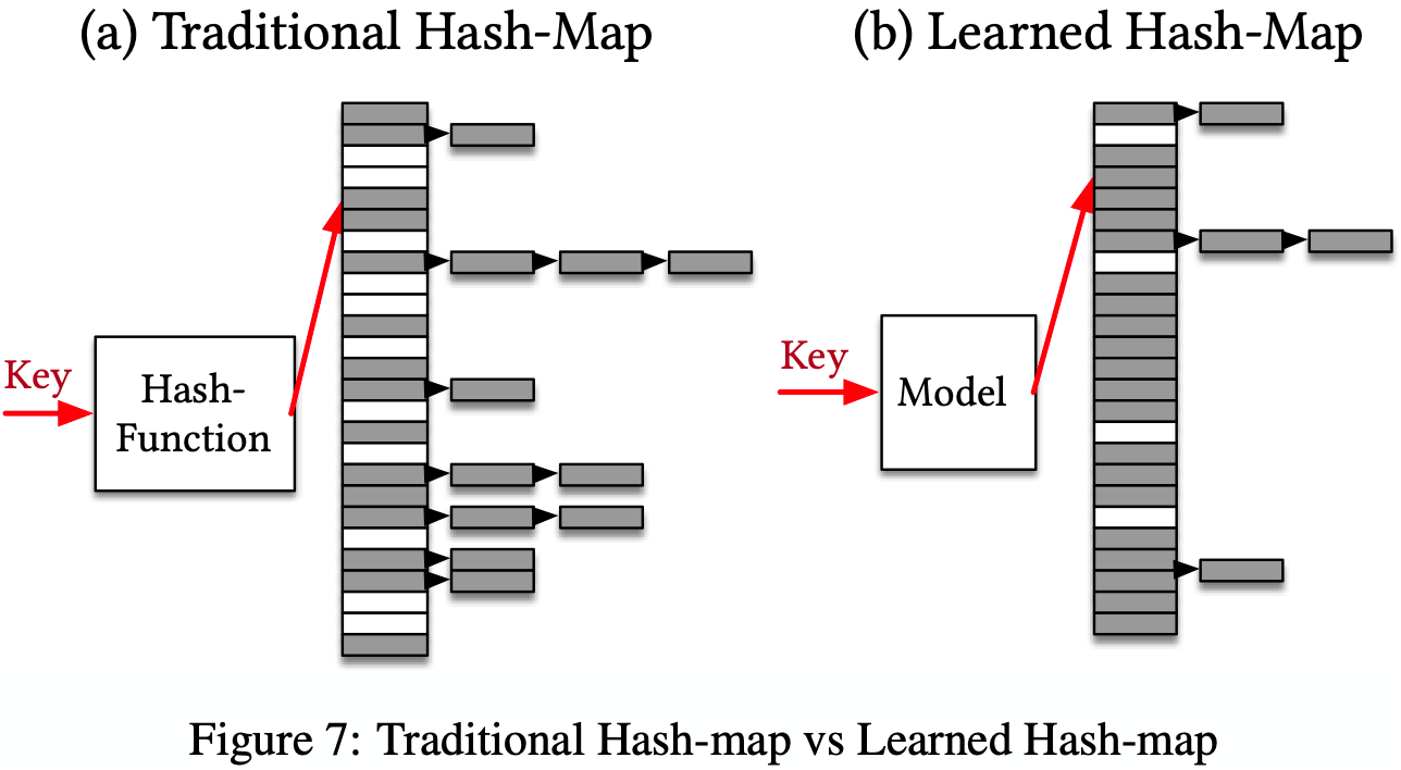
- Key challenge: prevent too many distinct keys from being mapped to the same position inside the Hash-map (i.e. a conflict)
- Learning the CDF of the key distribution is one potential way to learn a better hash function – records do not need to be stored compactly or in sorted order, but the CDF can be sclaed by the targeted size M of the Hash-map and use h(K ) = F (K ) ∗ M , with key K as our hash-function
- Recursive model architecture can be reused in this section – there is a trade-off between the size of the index and performance, which is influenced by the model and dataset
Results
Measure: conflict rate of learned hash functions over the three integer data sets (as previously shown)
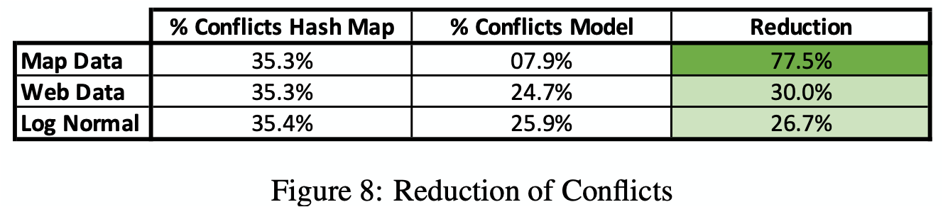
Results: learned models can reduce the number of conflicts by up to 77% over our datasets by learning the empirical CDF at a reasonable cost; the execution time is the same as the model execution time in Figure 4, around 25-40ns.
Limitations: the benefits from the reduction of conflicts is, given the model execution time, depends on the Hash-map architecture, payload, and many other factors
Existence Index
Bloom index and existence indexes are space efficient probabilistic data structure to test whether an element is a member of a set
Features
- Existence indexes need to learn a function that separates keys from everything else
- Highly space-efficient, but can still occupy a significant amount of memory
- High latency to access cold storage - more complex models can be built while the main objective is to minimize the space for the index and the number of false positives
Learned Bloom filters
- Objective: provide a specific False Positive Rate (FPR) for realistic queries in particular while maintaining a False Negative Rate (FNR) of zero
- Can make use of the distribution of keys nor how they differ from non-keys
- In considering the data distribution for ML purposes, we must consider a dataset of non-keys
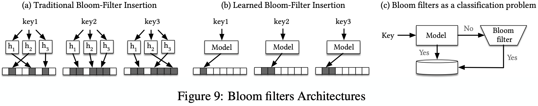
As a classification problem:
- The existence index is as a binary probabilistic classification task
o i.e. Learn a model f that can predict if a query x is a key or non-key
o Learned model can be fairly small relative to the size of the data - Learned model computation can benefit from machine learning accelerators
Bloom filters with Model-Hashes
- Learn a hash function with the goal to maximize collisions among keys and among non-keys while minimizing collisions of keys and non-keys
A comparison of Bloom Filters is shown below
Results
- Data taken from Google’s transparency report as our set of keys to keep track of, consisting of 1.7M unique URLs.
- Learned Bloom filter improves memory footprint at a wide range of FPRs. (Here W is the RNN width and E is the embedding size for each character.)
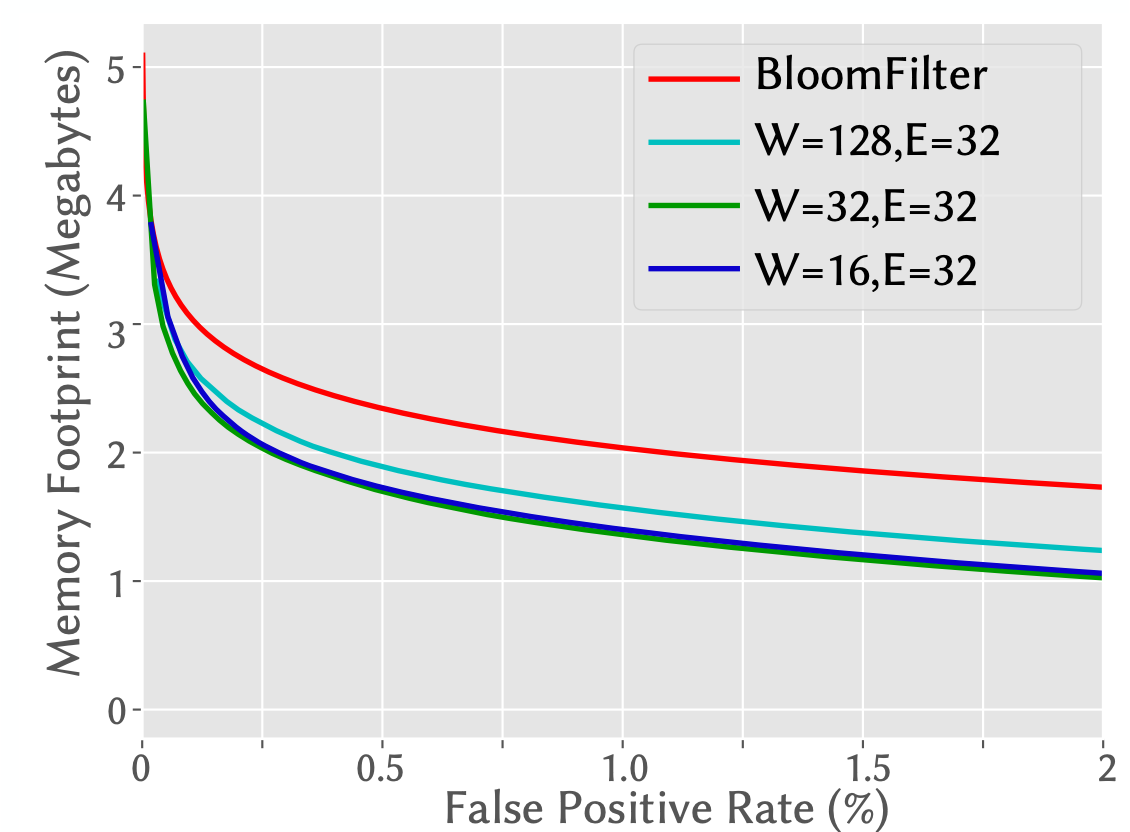
- A more accurate model results in better savings in Bloom filter size
- The model does not need to use the same features as the Bloom filter
Conclusion and Implications:
- Other ML Models: only linear models and neural nets were explored in this paper but many other ML model types and ways to combine them with traditional data structures are possible
- Multi-Dimensional Indexes: extending the idea of learned indexes to multi-dimensional indexes
- Beyond Indexing: Learned Algorithms: potential for a CDF model to speed-up sorting and joins, not just indexes
- GPU/TPUs: Can make the idea of learned indexes even more valuable, but present extra challenges such as high invocation latency and requires 2-3 micro-seconds to invoke any operation on them (however, integration of machine learning accelerators with the CPU is improving so techniques like batching requests the cost of invocation can be amortized, so invocation latency can be overcome)