Central limit theorem

Central limit theorem is an important theorem in statistics and probability. But before gaining more knowledge about it, let us first get to know about normal distribution and sampling from a distribution.

Table of contents:

1. Normal Distribution
2. Sampling from a distribution
3. Central limit theorem

Normal Distribution

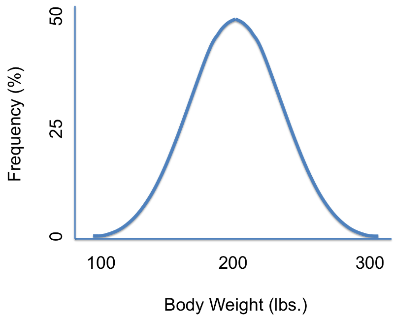
We might have seen the above type of graph in many places. It is known as a normal distribution or a Gaussian distribution. Since it is a symmetric curve that looks like a bell, it is also known as the "Bell shaped curve".

In the above example, the curve represents human body weight measurements. According to the graph, people can weigh 100 lbs (under weight) , 300 lbs (over weight) or 200 lbs (average weight). Practically, we do not find that many people who are malnourished or obese. So the frequency of these extremes are really low. On the same note, we find many people who are of average weight. Hence as we travel towards the average weight or mean from both the extremes, we find the curve to be rising and it reaches the maximum value at the mean.

The width of the curve represents the standard deviation.

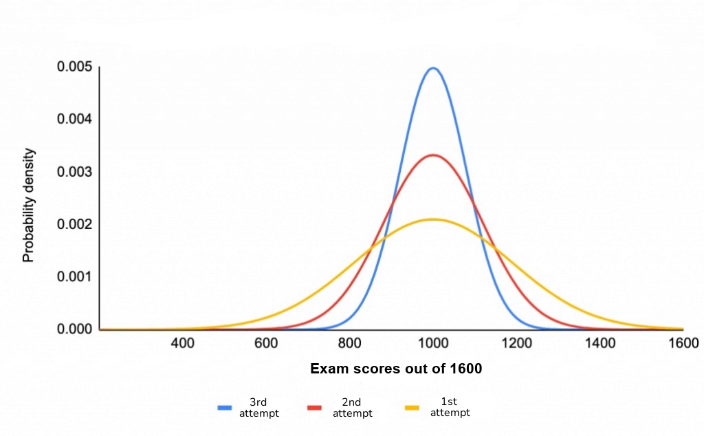
The graph shows the exam scores of students (out of 1600) in their first, second and third attempts. We find that the distribution curve narrows down as we increase the attempts and the peaks also sharpen. As increase the attempt, we find that the scores of students deviate less from 1000 (mean score). The width of the curve determines how tall it is: the narrower the curve, the taller.

Sampling from a distribution

As we already know, the tallest part of the distribution curve shows where the values occur more frequently and the values in the lower parts of the curve occur less frequently.

Sampling simply means picking out or selecting random values from the given curve based on their probabilities. In this digital era, this job is given to computers. For example, suppose we want the computer to pick one random value, there are high chances that it will pick a value from the tallest part of the curve. How ever at some times, it may also pick values from the lower ends of the curve. Usually the sample size is specified for the computer to generate random samples from the histogram or curve. The sample size denotes the number of entries that a sample should contain.

This sampling allows us to run statistical tests and compare our expected results to what will happen in reality.

Central limit theorem

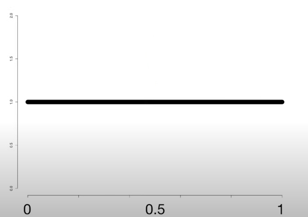
Let us consider a uniform graph shown below.

From the graph, let us select 20 samples and calculate its mean. The red line shows the mean of the selected samples.

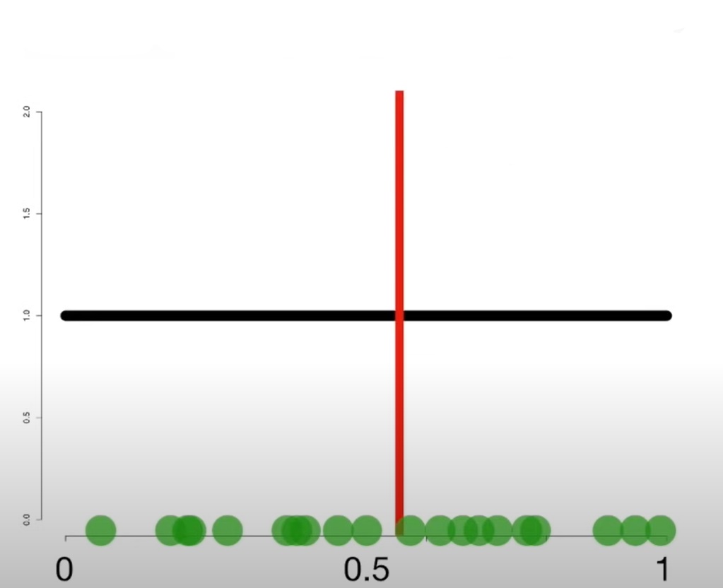
Then, let us plot the means we obtain as a histogram.

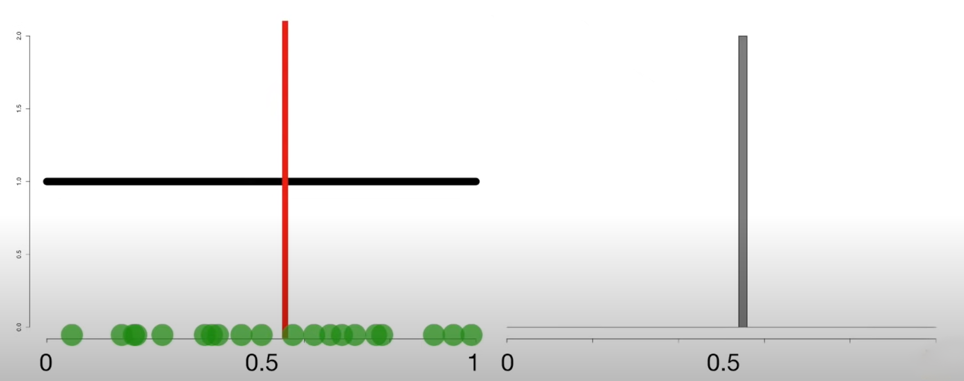
Now, let us collect 10 such samples and calculate the mean of each. At this stage, our histogram will look as shown.

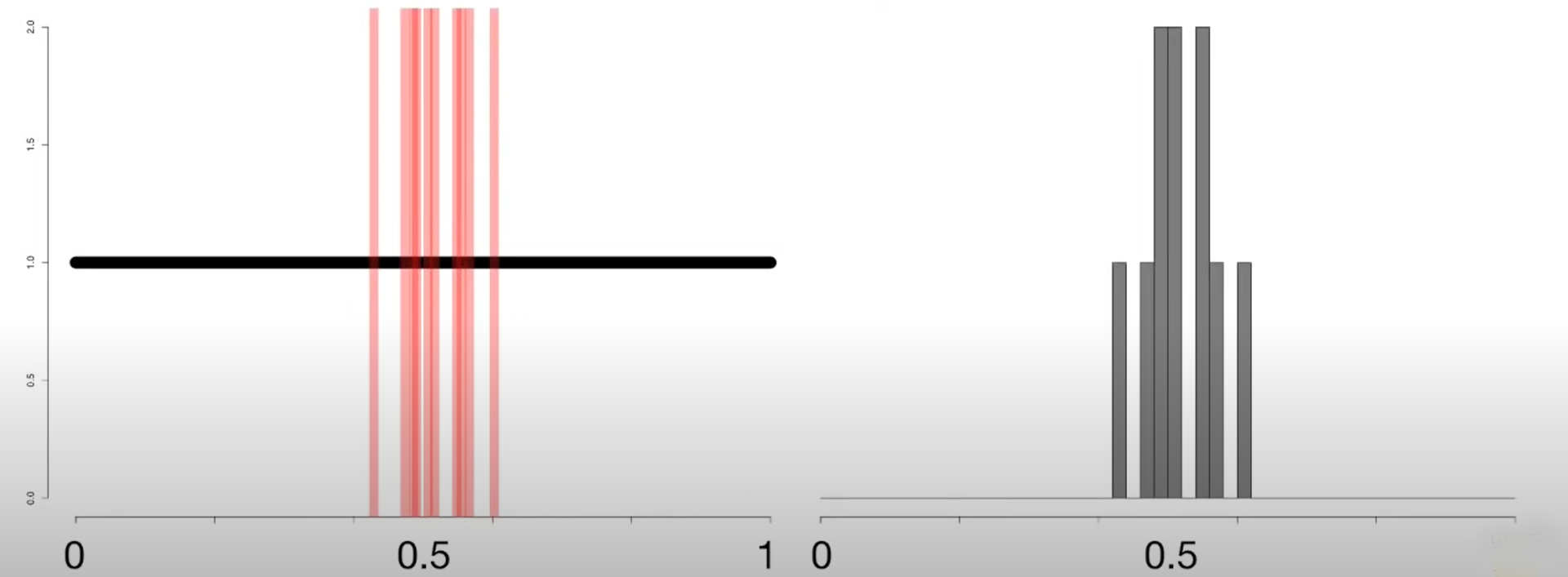
Now let us see how our histogram looks when 20,40,70 and 100 such samples and their means are taken.

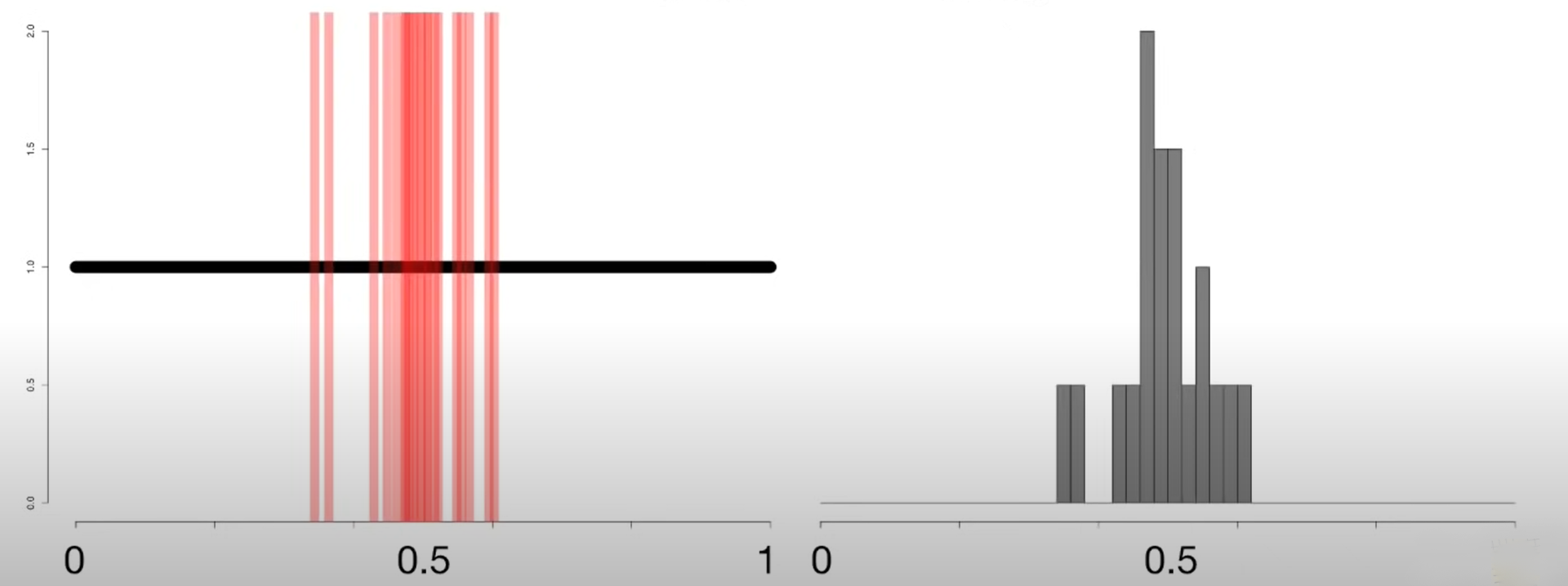
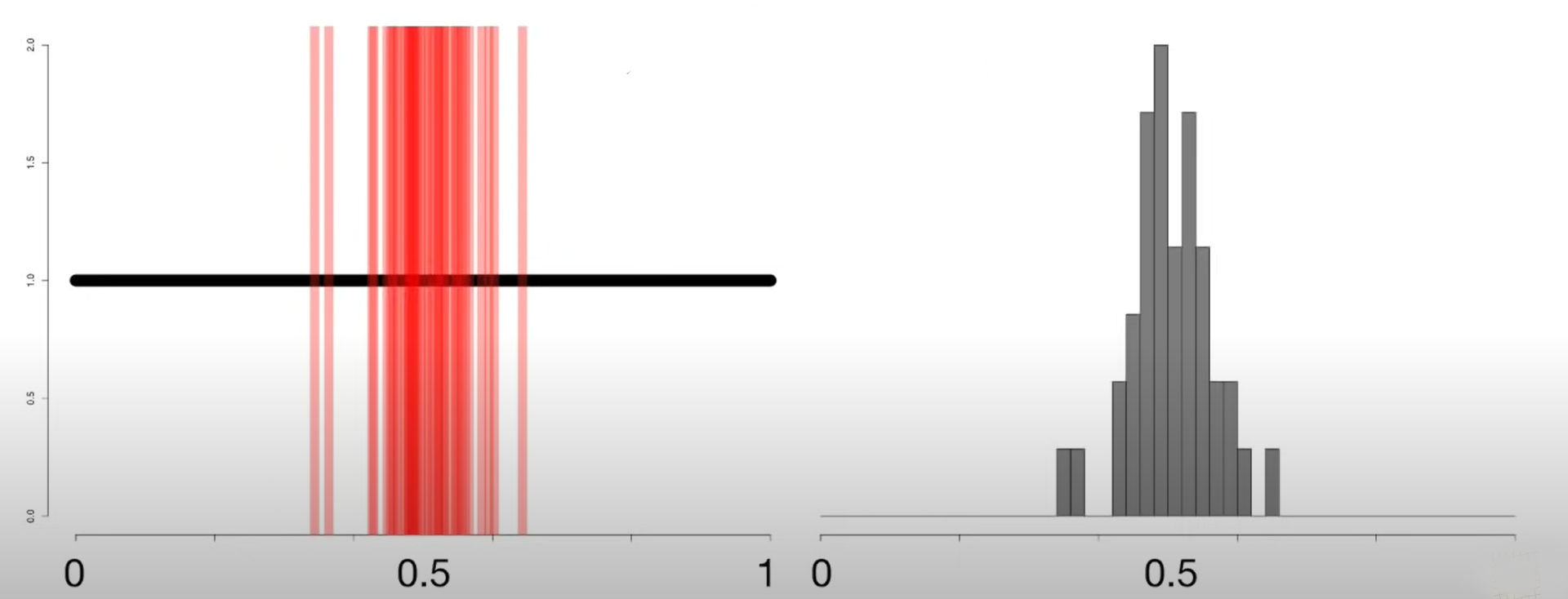
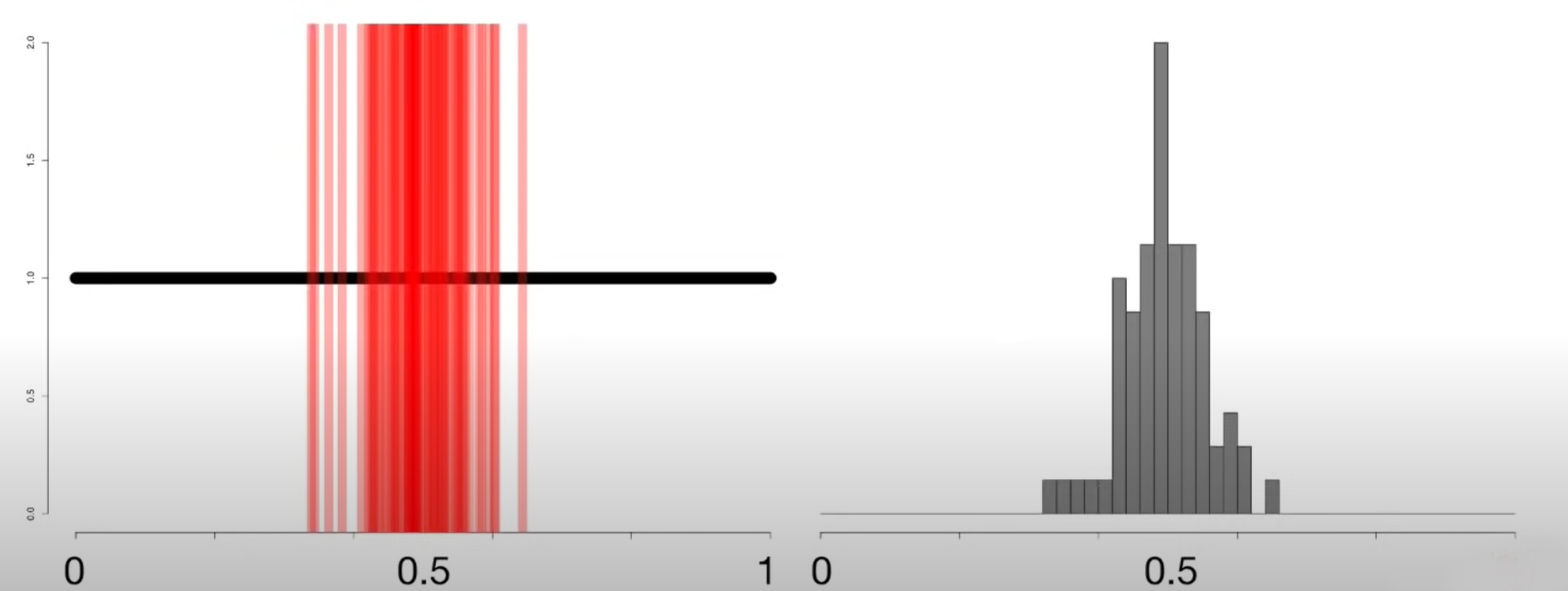
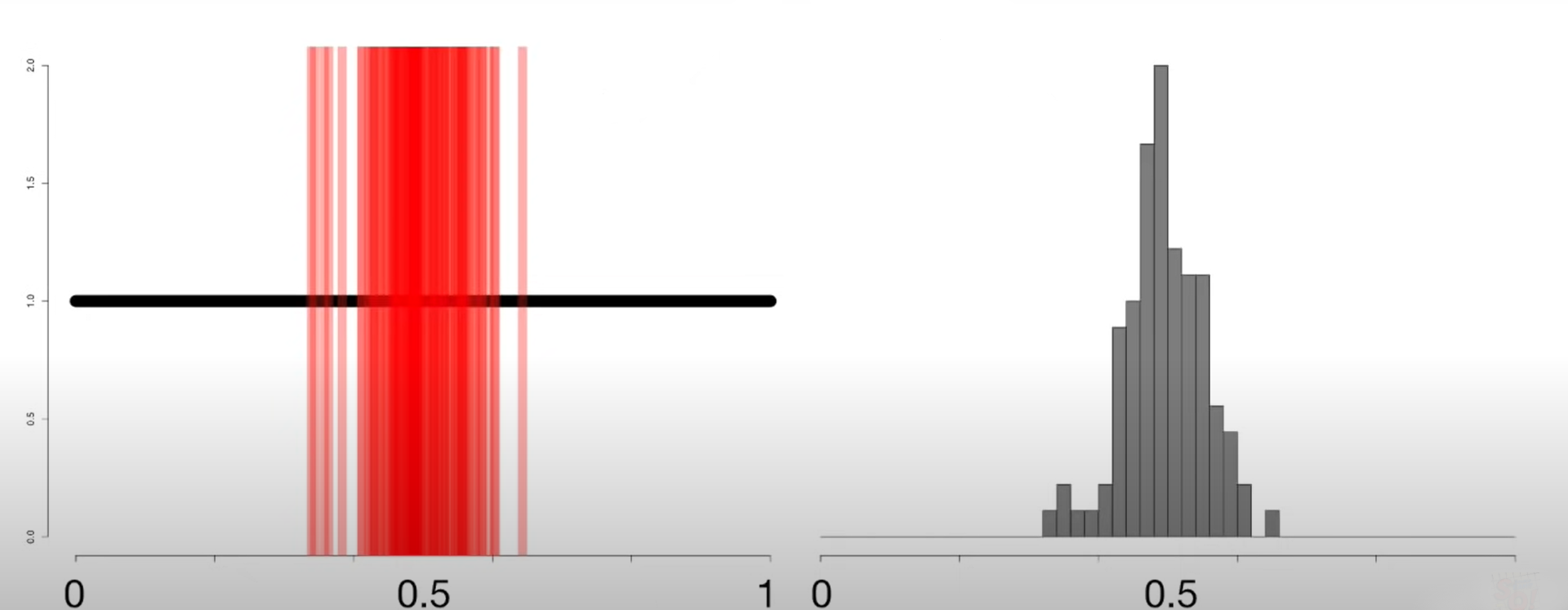
We notice that as we increase the number of samples, the histogram of means becomes more defined in the bell shape and a normal distribution curve can be easily overlayed on the histogram that we get when we consider 100 samples. This means that our means are normally distributed.

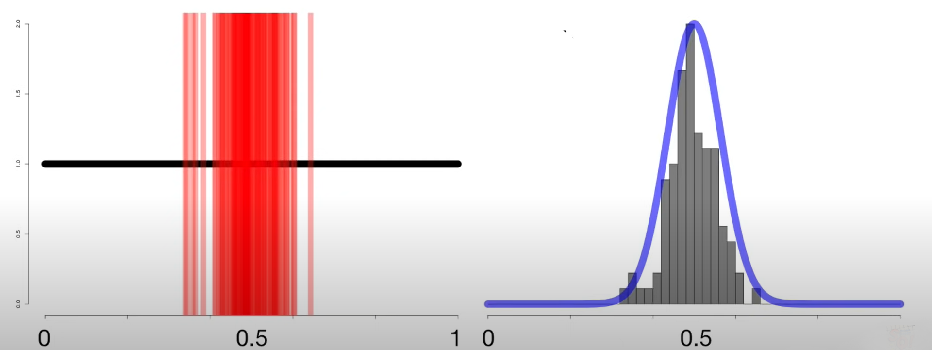
In the above case, we chose an uniform graph. But this pattern hold true for all types of graphs.

This is what the central limit theorem is all about! It states that "As the sample size becomes larger, the distribution of sample means approximates to a normal distribution curve."

Usually for this theorem to hold true, sample sizes equal to or greater than 30 are considered.

With this article at OpenGenus, you must have the complete idea of Central limit theorem.