
Problem: given an encoding of an image, to which extent is it possible to reconstruct the image itself?
Purpose and application of the inversion
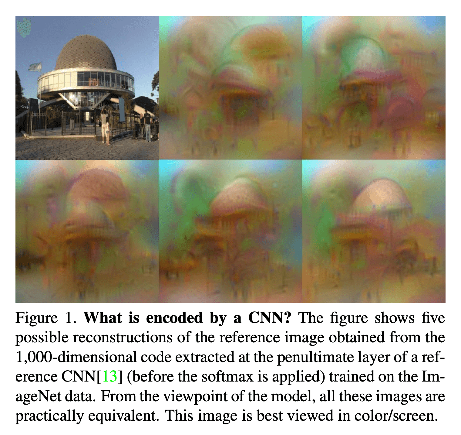
The study of the inverse of image representations give us the opportunity to see what is encided by a CNN. We can use invesion to reconstruct the output by layers in a CNN.
We have explored the paper "Understanding Deep Image Representations by Inverting Them" by Aravindh Mahendran and Andrea Vedaldi affiliated with University of Oxford.
Inversion Method
The paper presents a general method to invest representations, including those of SIFT, HOG and CNNs. This method only uses information from the image representation and a generic image.
The paper introduces their method of computing an approximate inverse of an image representation. The formula aims to find an image whose representation best matches the provided image.
Given the representation function

and the representation to be inverted

Reconstruction aims to find the image

which minimises the following equation.

where l represents the loss function that compare the two terms inside the brackets, with Phi(x) being the image representation and Phi0 being the target image. R is a regulariser caputring a natural image prior.
By minimising the equation the program outputs an image x* that resembles x0. As there might not be a unique solution, the program will output the possible reconstructions, which will help characterise the space of images that it thinks are equivalent.
Loss function
The paper elects to use the Euclidean distance for the loss function. The loss function may be modified in its nature to optimise selected neural responses.

The loss function is to be minimised by gradient descent.
Regulariser
The regulariser affects images by removing the details of the image. This paper elects to use total variation (TV), such that images consist of piece-wise constant patches.
It is given by  , where beta is 1.
As images are discrete, the TV norm can be represented by the following equation as the the TV norm has been replaced by the finite-difference approximation.

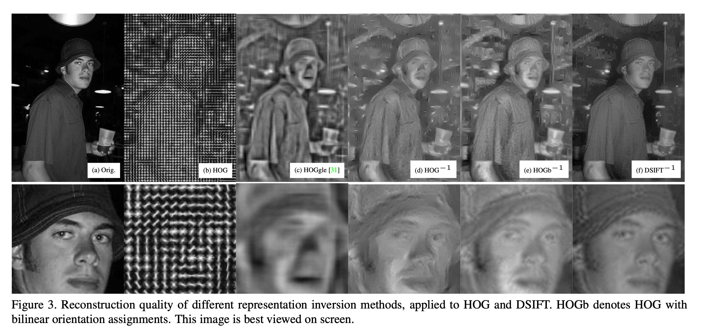
The key difference to using this equation is that it uses image priors, giving it the ability to recover low-level statistics removed by the representation. Compared to alternative reconstruction methods such as the Histogram of Oriented Gradients (HOG), this tool performs better. HOG divides the patches into blocks, then represents the gradient of each block with a histogram.
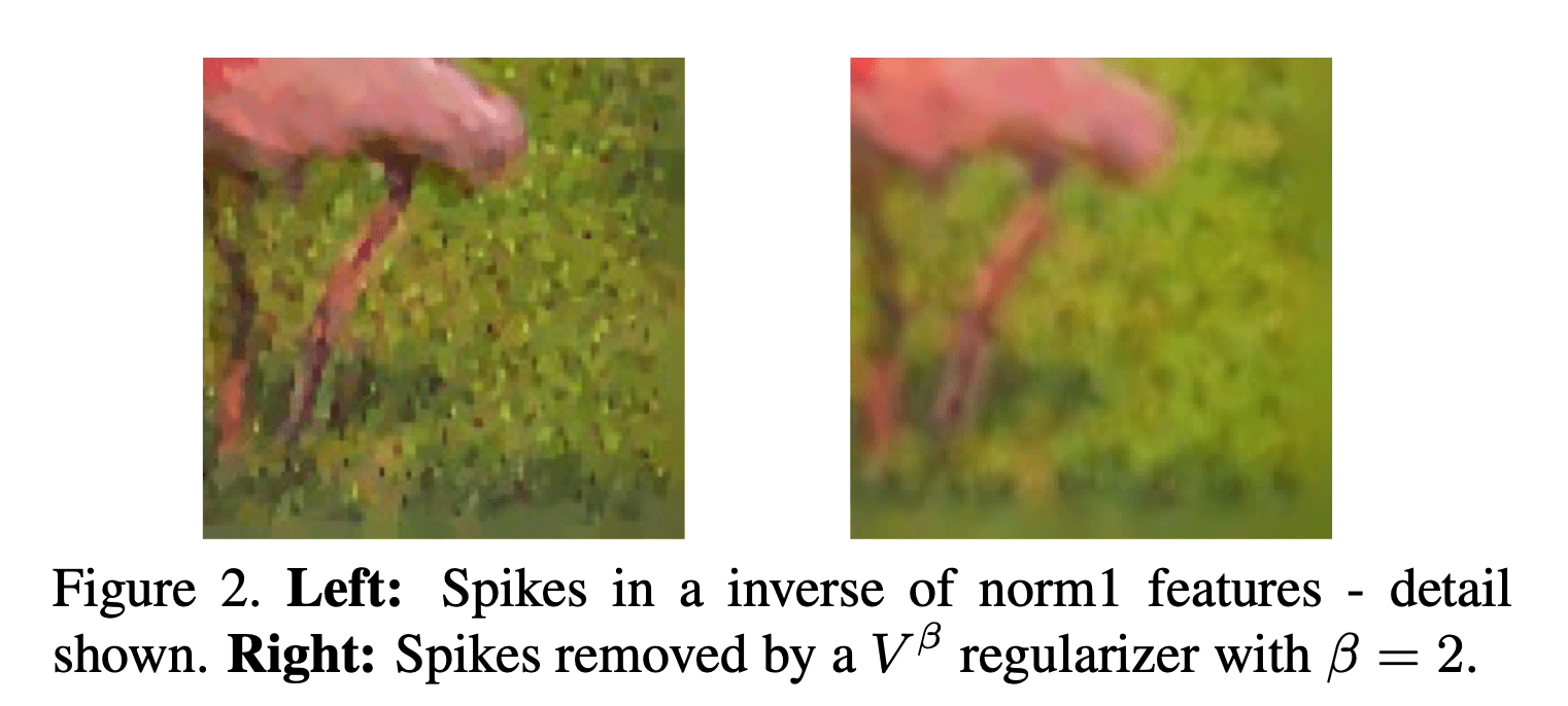
In using the TV regulariser, one outcome may be spikes in the reconstruction when inverting a layer of the network for instance. The spikes are located at specific points of the image. The causes of the particular locations of the spikes are attributed to first, the total variation norm along any path between two samples only depends on the overall amount of intensity change (it doesn't take into account the gradient, or the sharpness of the change). Furthermore, sharp changes are concentrated around a boundary with a small perimeter, for the changes to be optimally integrated on the 2D image.
Hence, there is a trade-off between the sharpness of the image and the removal of the spikes. By selecting a beta larger than 1, larger gradients are penalised, thus changes are distributed across regions instead of being concentrated in boundaries with small perimeters.
Balancing the Loss and Regulariser
By balancing the loss and regulariser, one can obtain an optimal tuning for the image.
First, the loss function should be replaced by the normalised version. The reason for this replacement is to fix the dynamic range of the function - the optimum can be expected to lie between [0, 1) and touch 0 at the optimum.
To compare the dynamic range of the regulariser, the solution should have a rougly unitary Euclidean norm. The first few laters of CNNS are sensitive to the scaling of the image range, as biases are tuned to a working range. Hence the objective with Phi(sigma x) should be considered, where sigma is the average Euclidean norm of natural images in a training set.
Furthermore, the alpha-norm regulariser must determine a suitable multiplier, such that the reconstructed image (sigma x) can be contained in a natural range.
The final form of the function can be considered as follows, 
Optimisation strategy
Despite deep representations being typically a chain of several non-linear layers and thus difficult to solve with optimisation, in this case the author illustrates the use of gradient descent. The gradient descent here is extended to use momentum so the learning time is significantly reduced. As gradient descent has been implemented, the derivatives of the loss function compared with the representation Phi have to be computed. By implementing HOG and DSIFT as CNNs, a particularly helpful CNN technique can be implemented - that of computing the derivative in each computational layer and composing the latter in an overall derivative of the function with back propagation.
Results
The paper experiments with both shallow and deep representations.
For experiments with shallow representations, HOG and DSIFT were used. Unfortunately, the direct implementation wasted significant resources as they used generic filtering code. With the optimisation of the implementation of the minimisation equation, perhaps it could require less time.
In the reconstruction of a deep representation, CNN-A, the first few layers were an invertible code of the image, then progressively became fuzzier, though they still maintained some similarity to the image. The CNN codes captured distinctive visual features of the original pattern, even the very deep layers.
Conclusion
In using image priors such as the V Beta normalisation, even low-level image statistics removed by the representation. Applying inversions can help visualise the information processed by each layer.