Reading time: 30 minutes | Coding time: 15 minutes

In Part 1 of our Reinforcement Learning Tutorial series, we learned about the basics of reinforcement learning, and also about one of the most easy algorithms to implement it, called Q-Learning.

Q-Learning was a greedy algorithm in that, the main strategy involved was to perform the action that will eventually yield the highest cumulative rewards.

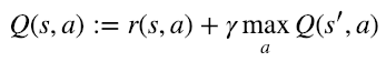
We also saw the Bellman equation, and how it forms the basis for Q-Learning.

If you want to refresh your concepts of Q-Learning, and get an intuitive introduction to how it all works, please refer to Part 1 of this series.

Now, let's get started with something at a little more advanced level - Deep Q-Learning!

Deep Q Networks

In Q-Learning, we made a table which had all the possible states as columns, and the actions which could be taken at every state as rows. But what would happen in an environment, where the number of states and possible outcomes would become very large?

Turns out, it's not rare, the possibility of this happening. Even a simple game such as Tic-Tac-Toe has hundreds of different states, which is then multiplied by 9, the number of possible actions.

So, how will vanilla Q-Learning help us solve complex problems like these?

The answer to this lies in Deep Q-Learning, an effort to combine Q-Learning and Deep Learning, the resultant being Deep Q Networks.

The idea is straightforward - where we had the table consisting of states and possible outcomes in Q-Learning, we'll now replace that with a neural network which tries to approximate Q Values, in Deep Q-Learning.
It's usually referred to as the approximator or the approximating function, and denoted as $Q\left(s, a; \theta \right)$, where $\theta$ represents the trainable weights of the network.

It makes sense to use the Bellman Equation here too, but what exactly are we minimizing? Let's take another peek at it:

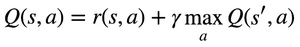
The "=" sign here stands for assignment, but do we have any condition which will also satisfy an equality?
Yes - when the Q Value reached its converged and final value.

And that is exactly our goal - so we could minimize the difference between the LHS and the RHS - to get our cost function.

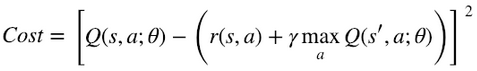
This might look familiar to your eyes, because it's the Mean Squared Error function, where the current Q Value is the prediction $\left(y\right)$, and the immediate, future rewards are the target $\left(y\text{'}\right)$:

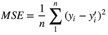
This is also why $Q\left(s\text{'}, a; \theta \right)$ is usually referred to as Q-target.

Let's move on to Training, now. In Reinforcement Learning, the training set is created on the fly - we ask the Agent to try and select the best action using the present network, and we record the state, action, reward and the next state it ended up at.

We zero on to a batch size $\left(b\right)$, and each time $\left(b\right)$ new records were recorded, we select $\left(b\right)$ records at random from the memory, to train the network.

The memory buffers are known as Experience Replay.

Many types of such memories exist - one of the most common is a Cyclic Memory Buffer, which makes sure the Agent keeps training over its new behavior rather than training on things that might no longer be relevant.

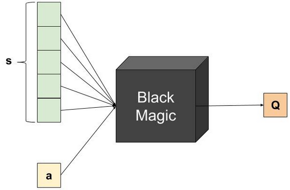
Talking about Architecture - if it's a table we're using, the network must receive the state and action as input, and should produce a Q-Value as output:

Despite being correct, this architecture is inefficient from a technical point of view.

Note that the cost function requires the maximal future Q-Value, so we'll need several network predictions for a single cost calculation.
Thus, we could use the following architecture instead:

Here, we provide the network with only the state $\left(s\right)$ as input, and receive Q Values for all possible actions at once.
This architecture is more efficient and much better than the previous one.

Congratulations, you just learned how Deep Q-Networks function!

Implementing a Deep Q-Network

To ensure smooth continuity of your understanding of Q Networks and Deep Q Networks, I'll demonstrate Deep Q Networks, starting from basic Q-Learning.

Here I'll share with you the full code and outputs, from scratch.

Importing the libraries and setting the seed

import random
import numpy as np
import pandas as pd
import tensorflow as tf
import matplotlib.pyplot as plt

from collections import deque
from time import time

seed = 23041974

random.seed(seed)
print('Seed: {}'.format(seed))

Game Design

The game the Q-agents will need to learn is made of a board with $4$ cells. The agent will receive a reward of $+1$ every time it fills a vacant cell, and will receive a penalty of $-1$ when it tries to fill an already occupied cell. The game ends when the board is full.

class Game:
  board = None
  board_size = 0
  
  def __init__(self, board_size = 4):
    self.board_size = board_size
    self.reset()
  
  def reset(self):
    self.board = np.zeros(self.board_size)
    
  def play(self, cell):
    ## Returns a tuple: (reward, game_over?)
    if self.board[cell] == 0:
      self.board[cell] = 1
      game_over = len(np.where(self.board == 0)[0]) == 0
      return (1, game_over)
    else:
      return (-1, False)

def state_to_str(state):
  return str(list(map(int, state.tolist())))
  
all_states = list()
for i in range(2):
  for j in range(2):
    for k in range(2):
      for l in range(2):
        s = np.array([i, j, k, l])
        all_states.append(state_to_str(s))
        
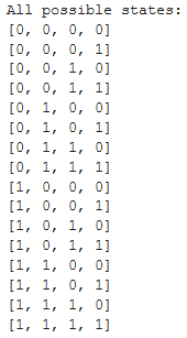
print('All possible states: ')

for s in all_states:
  print(s)

Initialize the game:

game = Game()

Q Learning

Starting with a table-based Q-learning algorithm

num_of_games = 2000
epsilon = 0.1
gamma = 1

Initializing the Q-table:

q_table = pd.DataFrame(0,
                       index = np.arange(4),
                       columns = all_states)

Letting the agent play and learn:

r_list = []    ## Store the total reward of each game so we could plot it later

for g in range(num_of_games):
  game_over = False
  game.reset()
  total_reward = 0
  while not game_over:
    state = np.copy(game.board)
    if random.random() < epsilon:
      action = random.randint(0, 3)
    else:
      action = q_table[state_to_str(state)].idxmax()
    reward, game_over = game.play(action)
    total_reward += reward
    if np.sum(game.board) == 4:    ## Terminal state
      next_state_max_q_value = 0
    else:
      next_state = np.copy(game.board)
      next_state_max_q_value = q_table[state_to_str(next_state)].max()
    q_table.loc[action, state_to_str(state)] = reward + gamma * next_state_max_q_value
  r_list.append(total_reward)
q_table

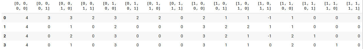
Let's verify that the agent indeed learned a correct strategy by seeing what action it will choose in each one of the possible states:

for i in range(2):
  for j in range(2):
    for k in range(2):
      for l in range(2):
        b = np.array([i, j, k, l])
        if len(np.where(b == 0)[0]) != 0:
          action = q_table[state_to_str(b)].idxmax()
          pred = q_table[state_to_str(b)].tolist()
          print('board: {b}\tpredicted Q values: {p} \tbest action: {a}\tcorrect action? {s}'
                .format(b = b, p = pred, a = action, s = b[action] == 0))

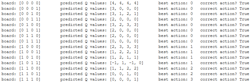
We can see that the agent indeed picked up the right way to play the game. Still, when looking at the predicted Q values, we see that there are some states where it didn't pick up the correct Q values.

Q Learning is a greedy algorithm, and it prefers choosing the best action at each state rather than exploring. We can solve this issue by increasing $\epsilon$ (epsilon), which controls the exploration of this algorithm and was set to $0.1$, OR by letting the agent play more games.

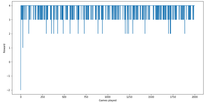
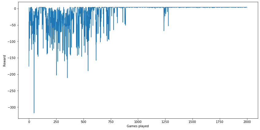
Let's plot the total reward the agent received per game:

plt.figure(figsize = (14, 7))
plt.plot(range(len(r_list)), r_list)
plt.xlabel('Games played')
plt.ylabel('Reward')
plt.show()

Deep Q Network

Let's move on to neural network-based modeling. We'll design the Q network first.

Remember that the output of the network, self.output is an array of the predicted Q value for each action taken from the input state, self.states. Comparing with the Q-table algorithm, the output is an entire column of the table.

class QNetwork:

  def __init__(self, hidden_layers_size, gamma, learning_rate,
               input_size = 4, output_size = 4):
    self.q_target = tf.placeholder(shape = (None, output_size), dtype = tf.float32)
    self.r = tf.placeholder(shape = None, dtype = tf.float32)
    self.states = tf.placeholder(shape = (None, input_size), dtype = tf.float32)
    self.enum_actions = tf.placeholder(shape = (None, 2), dtype = tf.int32)
    layer = self.states
    
    for l in hidden_layers_size:
      layer = tf.layers.dense(inputs = layer, units = 1,
                              activation = tf.nn.relu,
                              kernel_initializer = tf.contrib.layers.xavier_initializer(seed = seed))
                              
    self.output = tf.layers.dense(inputs = layer, units = output_size,
                                  kernel_initializer = tf.contrib.layers.xavier_initializer(seed = seed))
    self.predictions = tf.gather_nd(self.output, indices = self.enum_actions)
    self.labels = self.r + gamma * tf.reduce_max(self.q_target, axis = 1)
    self.cost = tf.reduce_mean(tf.losses.mean_squared_error(labels = self.labels,
                                                            predictions = self.predictions))
    self.optimizer = tf.train.GradientDescentOptimizer(learning_rate = learning_rate).minimize(self.cost)

Designing the Experience Replay memory which will be used, using a cyclic memory buffer:

class ReplayMemory:
  memory = None
  counter = 0
  
  def __init__(self, size):
    self.memory = deque(maxlen = size)
  
  def append(self, element):
    self.memory.append(element)
    self.counter += 1
    
  def sample(self, n):
    return random.sample(self.memory, n)

Setting up the parameters. Note that here we used gamma = 0.99 and not 1 like in the Q-table algorithm, as the literature recommends working with a discount factor of $0.9 \le \gamma \le 0.99$. It probably won't matter much in this specific case, but it's good to get used to this.

num_of_games = 2000
epsilon = 0.1
gamma = 0.99
batch_size = 10
memory_size = 2000

Initializing the Q-network:

tf.reset_default_graph()
tf.set_random_seed(seed)

qnn = QNetwork(hidden_layers_size = [20, 20],
               gamma = gamma,
               learning_rate = 0.001)
memory = ReplayMemory(memory_size)
sess = tf.Session()
sess.run(tf.global_variables_initializer())

Training the network. Compare this code to the above Q-table training.

r_list = []
c_list = []    ## Same as r_list, but for storing the cost

counter = 0    ## Will be used to trigger network training

for g in range(num_of_games):
  game_over = False
  game.reset()
  total_reward = 0
  while not game_over:
    counter += 1
    state = np.copy(game.board)
    if random.random() < epsilon:
      action = random.randint(0, 3)
    else:
      pred = np.squeeze(sess.run(qnn_output,
                                 feed_dict = {qnn.states: np.expand_dims(game.board, axis = 0)}))
      action = np.argmax(pred)
    reward, game_over = game.play(action)
    total_reward += reward
    next_state = np.copy(game.board)
    memory.append({'state': state, 'action': action,
                   'reward': reward, 'next_state': next_state,
                   'game_over': game_over})
    if counter % batch_size == 0:
      ## Network training
      batch = memory.sample(batch_size)
      q_target = sess.run(qnn.output, feed_dict = {qnn.states: np.array(list(map(lambda x: x['next_state'], batch)))})
      terminals = np.array(list(map(lambda x: x['game_over'], batch)))
      for i in range(terminals.size):
        if terminals[i]:
          ## Remember we use the network's own predictions for the next state while calculating loss.
          ## Terminal states have no Q-value, and so we manually set them to 0, as the network's predictions
          ## for these states is meaningless
          q_target[i] = np.zeros(game.board_size)
      _, cost = sess.run([qnn.optimizer, qnn.cost],
                         feed_dict = {qnn.states: np.array(list(map(lambda x: x['state'], batch))),
                                      qnn.r: np.array(list(map(lambda x: x['reward'], batch))),
                                      qnn.enum_actions: np.array(list(enumerate(map(lambda x: x['action'], batch)))),
                                      qnn.q_target: q_target})
      
      c_list.append(cost)
  r_list.append(total_reward)
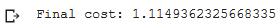
print('Final cost: {}'.format(c_list[-1]))

Again, let's verify that the agent indeed learned a correct strategy:

for i in range(2):
  for j in range(2):
    for k in range(2):
      for l in range(2):
        b = np.array([i, j, k, l])
        if len(np.where(b == 0)[0]) != 0:
          pred = np.squeeze(sess.run(qnn.output,
                                     feed_dict = {qnn.states: np.expand_dims(b, axis = 0)}))
          pred = list(map(lambda x: round(x, 3), pred))
          action = np.argmax(pred)
          print('board: {b} \tpredicted Q values: {p} \tbest action: {a} \tcorrect action? {s}'
                .format(b = b, p = pred, a = action, s = b[action] == 0))

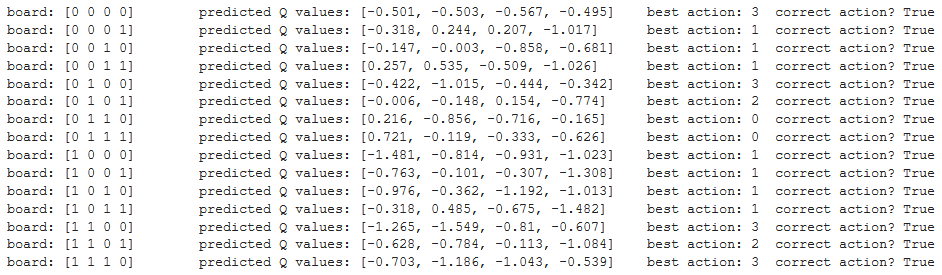
Here too, we see that the agent learned a correct strategy, and again, Q values are not what we would've expected.

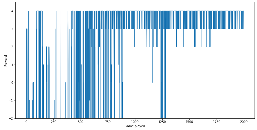
Let's plot the rewards the agent received:

plt.figure(figsize = (14, 7))
plt.plot(range(len(r_list)), r_list)
plt.xlabel('Games played')
plt.ylabel('Reward')
plt.show()

Zooming in, so we can compare the Q-table algorithm:

plt.figure(figsize = (14, 7))
plt.plot(range(len(r_list)), r_list)
plt.xlabel('Game played')
plt.ylabel('Reward')
plt.ylim(-2, 4.5)
plt.show()

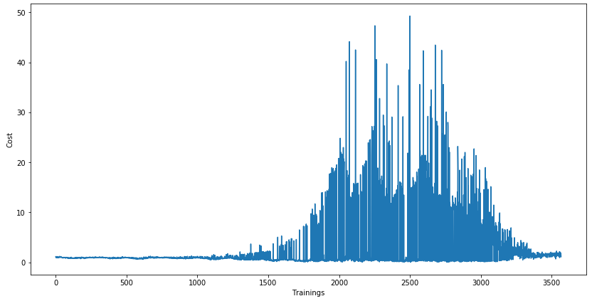
Let's plot the cost too. Remember that here the X-axis reflects the number of trainings, and not the number of games. The number of training depends on the number of actions taken, and the agent can take any number of actions during each game.

plt.figure(figsize = (14, 7))
plt.plot(range(len(c_list)), c_list)
plt.xlabel('Trainings')
plt.ylabel('Cost')
plt.show()

Bonus: You can play around with the code at this link.

That wraps up the demonstration of Q-Learning and Deep Q-Networks.
Hope you enjoyed this as much as I did.

Stay tuned for upcoming articles of the Reinforcement Learning Tutorial series!

Follow me on LinkedIn to get updates on more such intuitive articles.