
Reading time: 40 minutes | Coding time: 15 minutes
Around 6 years ago, in December 2013, a small and humble company in London called DeepMind Technologies uploaded their pioneering research paper, "Playing Atari with Deep Reinforcement Learning" to arXiv.
In the paper, they demonstrated how a computer which they trained, learned to play Atari 2600 video games by just observing the screen pixels and receiving a "reward" when the game score increased.
The games and the goals in every game were varied and designed to be challenging even for a human.
The results were remarkable as the same model architecture, without any changes made, was used to learn 7 different games, where the algorithm performed better than a human in 3 of them!
The paper and the algorithm (thanks to DeepMind) paved the way for General Artificial Intelligence, which is AI that can be utilized in a variety of environments, rather than being confined to strict realms such as driving a car or playing chess.
No wonder that DeepMind Technologies was immediately acquired by Google and has been on the forefront of deep learning research ever since.
DeepMind published an even better paper 2 years later, "Human-level control through deep reinforcement learning", which was featured on the cover page of Nature, one of the leading and coveted journals in the field of Science and Technology.
In this paper, they ==applied the same model to 49 different games and achieved superhuman performance in half of them!
The article you're leafing through now dear reader, is Part 1 of a series of upcoming articles on Reinforcement Learning topics.
We will give a basic introduction to Reinforcement learning in this article, and also tackle Q-Learning, along with an implementation in TensorFlow.
Excited? Let's begin!
An Introduction to Reinforcement Learning
Atari Breakout is one of the most famous video games I'm sure everyone in Gen-Z must have played in their childhood.
Fun Fact: The game was designed by Steve Wozniak and Steve Jobs, both being co-founders of Apple.
The game involves controlling a paddle at the bottom of the screen with the objective of bouncing a ball back to clear all the bricks situated in the upper half of the screen.
Each time you hit a brick, it disappears and your score increases, i.e. you get a reward.

Let's say we want to develop a neural network model to play this game.
The input to our network would be screen images, and output would be 3 actions: left, right or fire (to launch the ball).
You'd be right if you say that we can treat this problem as a classification one - for each game screen we have to decide whether we should move left, right, or press fire.
But wait. For that, we need lots and lots of training examples.
Sure, we could go and record game sessions of experts at this game, but that's not how we learn.
We don't need somebody to tell us a million times which move to choose at each screen.
We just need occassional feedback that what we did was the right thing, and can then figure out everything else ourselves.
This is where Reinforcement Leanring comes in. It lies somewhere between the domains of supervised and unsupervised machine learning.
While in supervised learning, we have a target label for each training example and in unsupervised learning, we have no labels at all, in reinforcement learning, we have sparse and time-delayed labels - our rewards.
Based on only these rewards, the agent has to learn how to behave in the environment.
There are multiple interesting problems related to reinforcement learning:
In Breakout, when we hit a brick and score a reward, it has nothing to do with the paddle movements (actions) we did just before getting the reward.
All the hard work was already done when we positioned the paddle correctly, and bounced the ball back.
This is known as the credit assignment problem - which of the preceding actions were responsible for getting the reward, and to what extent.
Once we have cracked the strategy to collect a certain number of rewards in the game, we are faced with a dilemma - should we stick to it or experiement with a new strategy which could result in even bigger rewards?
Let's take the example of Breakout again. A simple strategy is to move to the right edge and wait there.
When the ball is launched, it tends to fly right more often than left, which will result in us scoring 10 points each time before we die.
Should we be satisfied with this reward or should we do something to earn more rewards?
This problem is called the explore-exploit dilemma - should we exploit the known working strategy or explore other, possibly better and more efficient strategies.
Now let us define a typical Reinforcement Learning world.
Defining the World
A Reinforcement Learning task is all about training an Agent which interacts with its Environment.
The Agent transitions between different scenarios of the Environment, called states, by performing particular actions.
Actions, in return, yield rewards, which could be anything, but here let's assume we get points as rewards which could be positive, negative, or zero.
The objective of the Agent is to maximize the total reward it collects over an episode (everything that happens from the beginning of the initial start to the end of the terminal state).
We reinforce the Agent to perform specific actions by providing it with positive rewards, and to deviate from others by providing negative rewards.
This is how an Agent learns to develop a strategy, or policy.
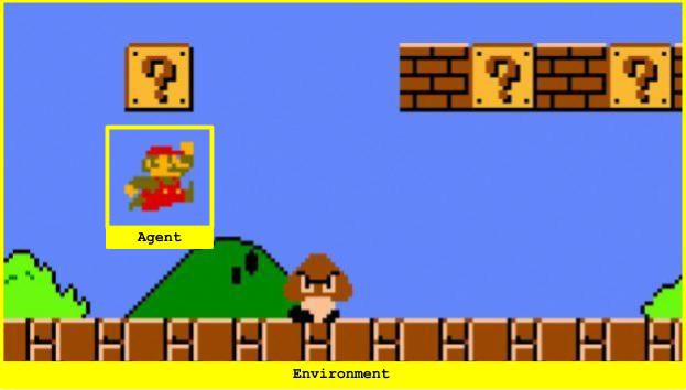
Taking another game as an example, let's understand the concept better using the environment of the Super Mario game.
Here, Mario is the Agent interacting with the world (the Environment).
The states are exactly what is visible on the screen, and an Episode is a level - the initial state is how the level begins, and the terminal state is how the level ends, whether we completed it or perished while trying.
The actions are move forward, move backwards, jump, etc.
When Mario collects coins or bonuses, it receives a positive reward, and when he falls or gets hit by an enemy, it receives a negative reward.
When he just wanders here and there, he receives no rewards, or a zero reward.
To be able to collect rewards, some arbitrary but essential actions are necessary to be taken - here, Mario has to walk towards the coins before he can collect them.
So, an Agent must learn how to handle postponed rewards (remember time-delayed labels we discussed above?) by learning to link those to the actions that actually caused them.
Now, let's take a peek at Markov Decision Processes, which form the backbone of Reinforcement Learning.
Markov Decision Processes
Each state the agent is in is a direct consequence of the previous state and the action previously performed.
The previous state is also a similar consequence of the one before that, and on it goes until we are left with the initial state.
Each one of these steps, and their order, hold information about the current state - and therefore have direct control on which action the Agent should choose next.
But we are faced with a problem - the further we go, the more information the Agent needs to save and process at every given step it takes.
This can quickly become unfeasible, due to the inability to perform calculations.
As a solution to this problem, we assume that all states are Markov States, that is, any state solely depends on the state that came before it (the action performed), and the transition from that state to the current one (the reward given).
Have a look at these 2 Tic-Tac-Toe games:
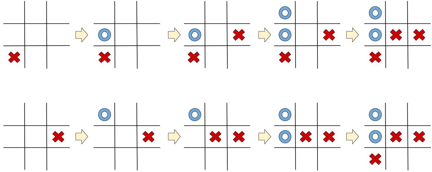
The final state reached in both the games is exactly the same, but the steps taken to reach there are different for both.
In both cases, the blue player must capture the top-right cell, or he will lose.
All we needed in order to find this was the last state, nothing else.
Note that, when using the Markov assumption, data is being lost - this becomes important in complex games such as Go or Chess, where the order of the moves hold implicit information about the opponent's strategy or way of thinking.
Nevertheless, the Markov states assumption is fundamental when attempting to calculate long-term strategies.
The Bellman Equation
Let's assume we already know what is the expected reward for each action at every step.
How do we choose which action to perform in this case?
Simple. We choose the sequence of action which will eventually generate the highest reward.
Q-Value (a.k.a. Quality Value) is the name given to the cumulative reward we will receive.
It can be mathematically stated as follows:
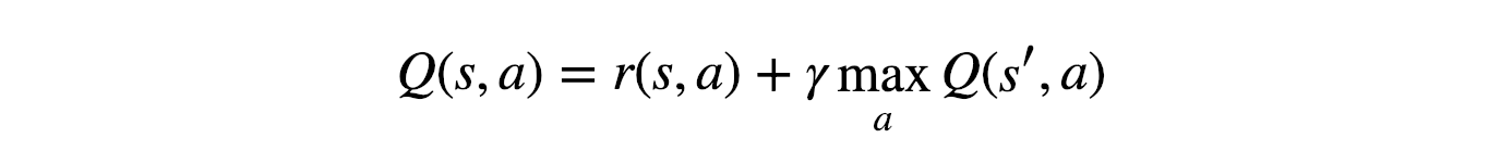
The equation above conveys that the Q-Value yielded from being at state s and selecting action a, is the immediate reward received, r(s, a), added to the highest Q-Value possible from state s' (the state the agent ended up after taking action a from state s).
How do we receive the highest Q-Value from s'?
By choosing the action that maximizes the Q-Value.
is the discount factor, which controls the importance of long-term rewards vs. the immediate one.
The equation we saw just now is the famous Bellman equation, its Wikipedia page provides a thorough explanation of how its mathematically derived.
This equation is quite powerful and is of huge importance to us due to 2 important characteristics:
-
While we are still preserving the Markov States assumptions, the recursive nature of the Bellman Equation allows rewards from future states to propagate to far-off previous states.
-
It is not necessary that we know the true Q-Values when starting. Since the equation is a recursive one, we can guess arbitrary values and it will eventually converge to the real ones.
Having collected everything we needed to understand Q-Learning in our rucksack, let's tackle the main boss: Q-Learning!!
Q-Learning
Let's recapitulate our strategy.
Our strategy is that, at any given state, we have to perform the action that will eventually yield the highest cumulative reward.
Q-Learning is thus, a greedy algorithm.
One method to implement Q-Learning to solve real-world problems is to draw a table to store all possible state-action combinations, and use it to save and update the Q-Values after every iteration.
We can update the values using the Bellman Equation :
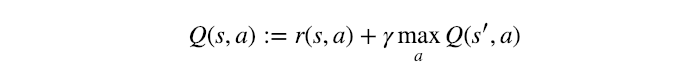
The above equation can be called the Q-Learning update rule for regular states.
The ":=" notation is used to explicitly denote assignment, and not equality.
Let's understand it better using a demonstration.
Some states are terminal states too. When the Agent reaches such a state, no actions or state-transitions are possible.
So, if the future state s' is a terminal state, we should use the following equation:
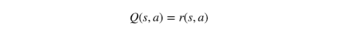
This is the Q-Learning update rule for terminal state s'
You might be thinking that we have reached the solution, but we are not done yet!
The greedy algorithm we devised has a serious problem - if we keep selecting the best actions, we'll never try anything new, and might miss a more rewarding approach just because we never tried it.
As a solution, we'll use the -greedy approach: for some , we choose the greedy action (by looking up our table) with a probability , or a random action with probability .
By doing this, we are giving the Agent a chance to explore new possibilities.
Congratulations! We are done understanding what Q-Learning is, our very first Reinforcement Learning algorithm.
Q-Learning demonstrations (using TensorFlow)
Using TensorFlow, we'll implement Q-Learning on a simple game of filling a 4 x 1 board.
A) Importing the libraries
import random
import numpy as np
import pandas as pd
import tensorflow as tf
import matplotlib.pyplot as plt

from time import time
Next, we choose a seed so that our performance can be reobtained in the future.
seed = 2205
random.seed(seed)

print('Seed: {}'.format(seed))
B) Game Design
There exists a board with 4 cells.
The Q-agent will receive a reward of +1 every time it fills a vacant cell,
and will receiev a penalty of -1 if it tries to fill an already occupied cell.
The game ends when the board is full.
class Game:

  board = None
  board_size = 0

  def __init__(self, board_size = 4):
    self.board_size = board_size
    self.reset()

  def reset(self):
    self.board = np.zeros(self.board_size)

  def play(self, cell):
    ## Returns a tuple: (reward, game_over?)
    if self.board[cell] == 0:
      self.board[cell] = 1
      game_over = len(np.where(self.board == 0)[0]) == 0
      return (1, game_over)
    else:
      return (-1, False)
def state_to_str(state):
return str(list(map(int, state.tolist())))
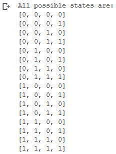
all_states = list()
for i in range(2):
for j in range(2):
for k in range(2):
for l in range(2):
s = np.array([i, j, k, l])
all_states.append(state_to_str(s))
print('All possible states are: ')
for s in all_states:
print(s)
Let's initialize the game now:
game = Game()
C) Q-Learning
num_of_games = 2000
epsilon = 0.1
gamma = 1
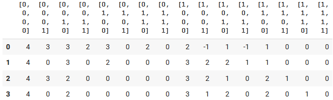
Initializing the Q-Table:
q_table = pd.DataFrame(0,
                       index = np.arange(4),
                       columns = all_states)
Letting the agent play and learn:
r_list = []  ##Stores the total reward of each game so we can plot it later

for g in range(num_of_games):
  game_over = False
  game.reset()
  total_reward = 0

  while not game_over:
    state = np.copy(game.board)
    if random.random() < epsilon:
      action = random.randint(0, 3)
    else:
      action = q_table[state_to_str(state)].idxmax()

    reward, game_over = game.play(action)
    total_reward += reward
    if np.sum(game.board) == 4:  ##Terminal state
      next_state_max_q_value = 0
    else:
      next_state = np.copy(game.board)
      next_state_max_q_value = q_table[state_to_str(next_state)].max()
    q_table.loc[action, state_to_str(state)] = reward + gamma * next_state_max_q_value
  r_list.append(total_reward)
q_table
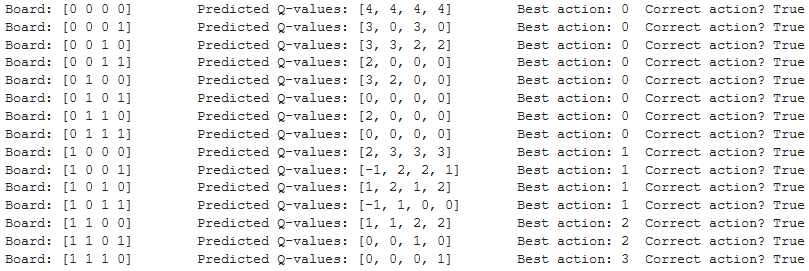
Let's verify that the agent indeed learnt a correct strategy by seeing what action it will choose in each one of the possible states
for i in range(2):
  for j in range(2):
    for k in range(2):
      for l in range(2):
        b = np.array([i, j, k, l])
        if len(np.where(b == 0)[0]) != 0:
          action = q_table[state_to_str(b)].idxmax()
          pred = q_table[state_to_str(b)].tolist()
          print('Board: {b}\tPredicted Q-values: {p}\tBest action: {a}\tCorrect action? {s}'.format(b = b, p = pred, a = action, s = b[action]==0))
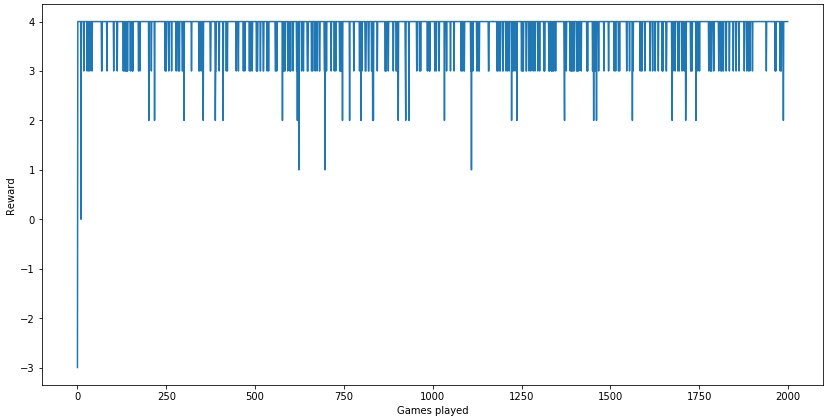
We can improve the performance of our algorithm by increasing the (epsilon) value (which controls how much the algorithm can explore), or by letting the agent play more games.
Let's plot the total reward the agent received per game:
plt.figure(figsize = (14, 7))
plt.plot(range(len(r_list)), r_list)
plt.xlabel('Games played')
plt.ylabel('Reward')
plt.show()
You could interact and play with the code here.
So that's a wrap, dear reader. This was part 1 of the Reinforcement Learning Tutorial series.
I hope I have given a lucid explanation of Reinforcement Learning and related topics. Hoping that you are now thorough with the concept of Q-Learning.
In the next article, we'll talk about Deep Q-Learning.