Denoising Autoencoders (DAEs)

Overview

The aim of this article is to discuss the Denoising Autoencoder (DAE) in sufficient detail. Hopefully, by the end of the article, readers would have obtained an understanding of the denoising autoencoder.

---

Table of Contents

The article is delineated into a set of sections. These are outlined below.

1. Justification for Autoencoders (AE)
2. What are Autoencoders?
3. DAEs as Autoencoders (i.e. the AE in DAE )
4. Application of DAEs
5. Question
6. Practicum and Implementation
7. Resources
8. Conclusion

---

Justification for Autoencoders

The field of machine learning, as befits a subset of Artifiial Intelligence, is concerned with building machines that can carry out cognitive tasks in human-like fashion. This is, however, easier said than done, for a number of reasons.

First, humans have a large body of background knowledge at our disposal. Even more fascinating, we have little conscious knowledge of how this came to be! As an instance, we really do not know how we learn our mother tongues. We just grow up to speak them! (Apparently).

Secondly, not all information we have is actually important. Humans have evolved to be able to discern the importance of different sources and/or objects of information. We are capable of ranking the different particulars of a situation, and making decisions regarding the more important particulars for a given situation. This is of even more importance today, in a world where we experience a serious barrage of information at an astounding rate.

Thirdly, and in the same vein as the second point above, storage solutions though cheaper than they used to be, are still quite expensive. Wouldn't it be great if we could store the important information without having to bother about the other not-so-important bits?

All these and more give rise to a very interesting solution: Autoencoders.

---

What are Autoencoders?

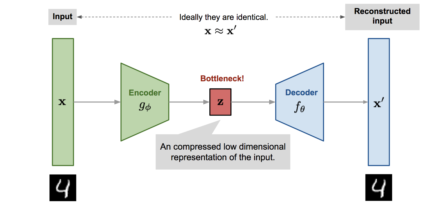
Autoencoders are neural networks designed to obtain a compressed summary of data. This is a fancy way of saying that the autoencoder is designed to understand the underlying intricacies that make up the data. The compressed summary learned is the "essence" of the data, and ideally, having this summary would allow us to recover the data.

According to Wikipedia:

An autoencoder is a type of artificial neural network used to learn efficient codings of unlabeled data (unsupervised learning). The encoding is validated and refined by attempting to regenerate the input from the encoding.

Imagine all the things we can do with this summary (code, in autoencoder parlance)!. Things like data compression, clustering, and dimensionality reduction become much more interesting! However, this article is about a specific kind of autoencoder: the Denoising Autoencoder (DAE).

Figure 1. : An Autoencoder

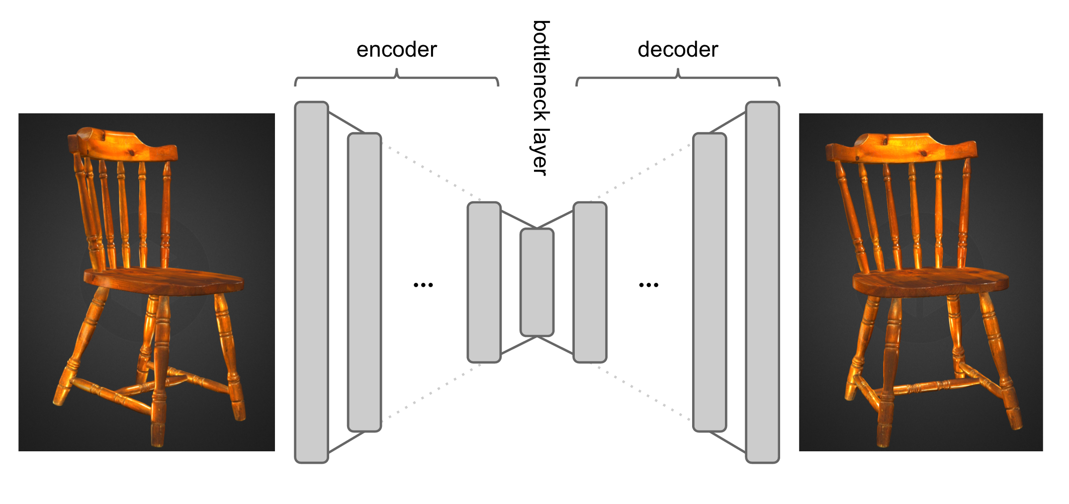
The autoencoder architecture is designed as a composite of two main parts: the Encoder and the Decoder. As inferrable from the name, the Encoder tries to learn a coded summary of the data, or an encoding, which would be (a.) more condensed and, (b.) of smaller dimensionality than the actual data. Provided the Encoder does its job well, it is the job of the Decoder to learn how to reconstruct the data (as perfectly as possible) from the coded summary.

Figure 2. : Convolutional Autoencoder Architecture

This is very similar to the old "compress-decompress" process with dear "WinRAR", a popular data compression solution. If we compress and then decompress a file, we should end up with the same file, and the intermediate compressed file (analogous to the encoding produced by an autoencoder's encoder) must be of a smaller size than the original data.

---

DAEs as Autoencoders

Like any other autoencoder, the DAE is designed to learn the innate structure (i.e. summary) of data. The DAE, however, goes an extra step. It attempts to divine this innate structure, and do so in such a thorough manner that, when faced with a corrupted (or noisy) version of the data, it can eliminate most, and ideally, all, of the corruption in the data. By noise, we mean artefacts in our data that may be due to:

• Malfunctioning sensors
• Quantization
• Damage over time (e.g. old images)

This denoising/reconstruction process is illustrated via Figure 3. below:

Figure 3. : Denoising Autoencoder Architecture

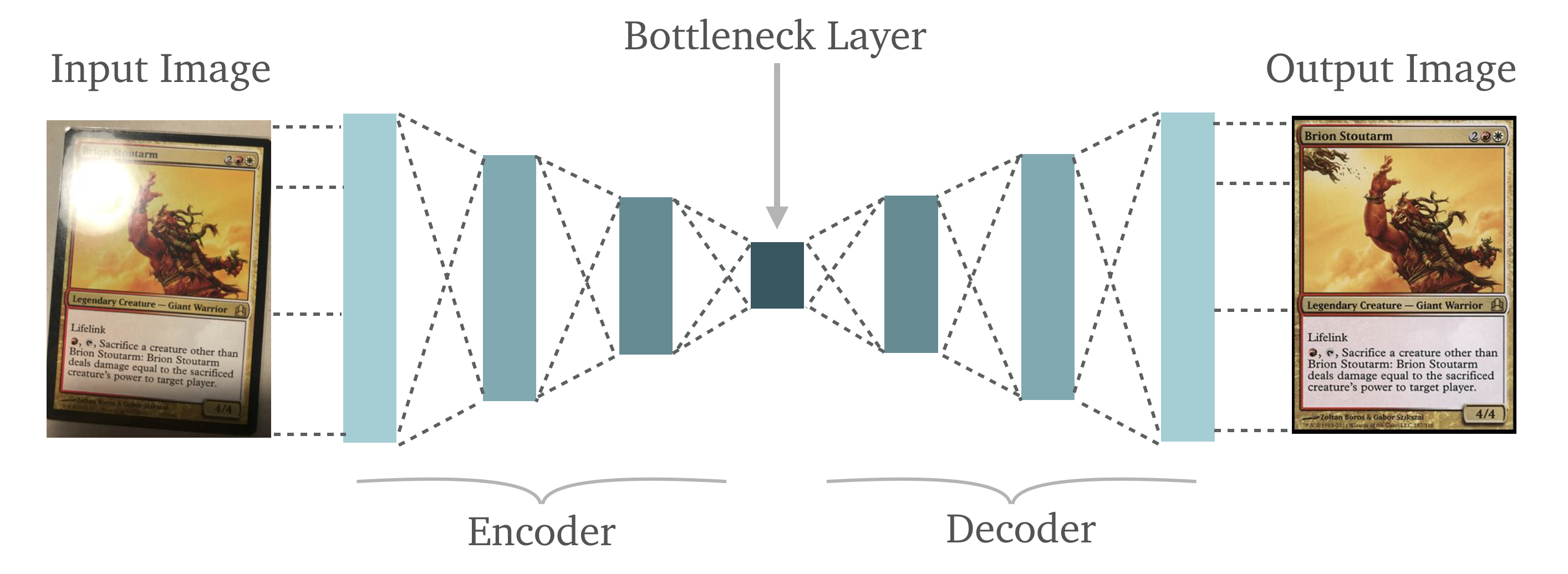
The input data (a corrupted version of the actual data) is passed into the Encoder to produce the encoding (also called bottleneck, code or embedding). This embedding is then passed into the Decoder, which reconstructs the data via the embedding.

Note the upper left corners of both the input image and the reconstructed image depicted above in Figure 3. This is a very good illustration of what a DAE is capable of.

At this juncture, however, it should be noted that denoising was NOT the original intent behind the design of the DAE. The denoising autoencoder was the by-product of attempts to improve the generalization ability of the vanilla autoencoder (AE), via a regularization technique known as Noise Robustness, which is similar to data augmentation, at least in principle.

The justification for this modification was that the easiest means for the autoencoder to reconstruct the inputs would be to use the identity function:

$$\text{ {X} = {X}{I_n} }$$
$$\mathrm{X} = \mathrm{I_n}\mathrm{X}$$
$$\text{where, X = data, }\mathrm{I_n} = \text{Identity matrix}$$

Data corruption via noise was postulated as a viable means of preventing this state of affiars, thus forcing the autoencoder to actually learn from the data, instead of just copying the input over to the output via the identity function as discussed earlier.

It just so happens that in the process of learning the data representation irrespective of noise, the DAE also learns to differentiate the noise from the legitimate signal. As such, DAEs tend to be better at representation learning than vanilla AEs.

---

Practicum and Implementation

Now that we have a satisfactory understanding of the DAE, its time we delved into some code. We will require some necessary and optional dependencies for this.

Necessary packages include:

• Tensorflow
• Matplotlib

Optional packages include:

• os (directory access)
• jupyterthemes (for aesthetics)

We begin by importing our required libraries: tensorflow, matplotlib. We also import other required utilities.

import os
import tensorflow as tf

from matplotlib import pyplot as plt
from jupyterthemes import jtplot

from tensorflow.keras.utils import image_dataset_from_directory

from tensorflow.keras import layers
from tensorflow.keras import Sequential, Model

from tensorflow.keras import losses
from tensorflow.keras import optimizers

jtplot.style('gruvboxd')

For this implementation, we will be making use of the wildly-popular Fashion-MNIST dataset. This dataset comprises of fashion articles which fall into one of ten categories:

• Ankle boot
• Bag
• Coat
• Dress
• Pullover
• Sandal
• Shirt
• Sneaker
• T-shirt
• Trouser

Using the keras subpackage in tensorflow would allow us to load the data easily:

(X_train, _), (_, _) = tf.keras.datasets.fashion_mnist.load_data()

However, in the interest of learning how to load data from local (we can't always have ready-made data on the net, can we?), we will use another keras functionality: image_dataset_from_directory. It takes the following arguments:

• Directory (where is the dataset located?)
• Batch size
• Color mode (rgb, rgba, or grayscale)
• Image size (desired size for images)
• Labels (whether or not to load accompanying labels for images)

We use the function like so:

### Import image data the data from local storage
X_train = image_dataset_from_directory(DATA_DIR, labels = None,
                                       color_mode = 'grayscale',
                                       image_size = (28, 28),
                                       batch_size = 32)

Running the function above returns a tf.data.Dataset object. This object is optimized for tensorflow data opereations, and is one of the recommended formats for storing image data.

We can confirm this by typechecking:

### Type of data object
print(type(X_train))

Output:

<class 'tensorflow.python.data.ops.dataset_ops.BatchDataset'>

We need to scale the data from the range [0., 255.] to range [0., 1.]. We do this by taking advantage of the map property:

### Scale Dataset
X_train = X_train.map(lambda x: x/255., num_parallel_calls = 3)

We can confirm that the X_train object iteratively returns our data:

### Get a new batch of data out of the scaled iterator
X = next(iter(X_train))

To round it off, we can package the whole data preparation process as a function:

### Data preparation in one go
def prepare_data(data_dir, batch_size = 32, image_size = (28, 28)):
    
    ''' Load the image data as a tf.data.Dataset object.'''
    
    data = image_dataset_from_directory(data_dir, batch_size = batch_size,
                                        image_size = image_size, labels = None,
                                        color_mode = 'grayscale')
    data = data.map(lambda x: x/255., num_parallel_calls = 3)
    
    return data

And we can simultaeneously load and prepare the data using this function, like so:

### Load and prepare data
X_train = prepare_data(DATA_DIR, batch_size = 64)

We also define a function to assist in visualizing the images (both actual images and their noisy version).

### Visualize each image in the real batch
def visualize(data, nrows = 4, ncols = 8):
    
    ''' Visualize images. '''
    
    fig, ax = plt.subplots(nrows = nrows, ncols = ncols, figsize = (20, 10))
    i = 0
    for r in range(nrows):
        for c in range(ncols):
            ax[r,c].imshow(data[i].numpy().squeeze())
            i += 1
    
    #plt.grid(False)
    plt.show(); plt.close('all')
    
    return None

Now we can visualize our images. We visualize an actual batch of images, and we also visualize the batch when it is corrupted with Gaussian noise.

Input I (Image batch):

### Visualize actual batch
visualize(data = X)

Input II (Corrupted image batch):

### Visualize corrupted batch
visualize(data = X + tf.random.normal(mean = 0., stddev = 0.1, shape = X.shape))

The resulting images are as below:

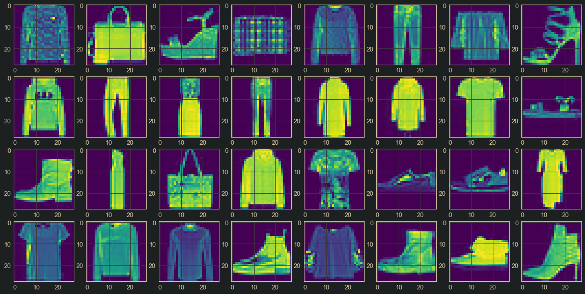
Figure 4. : Actual Image Batch

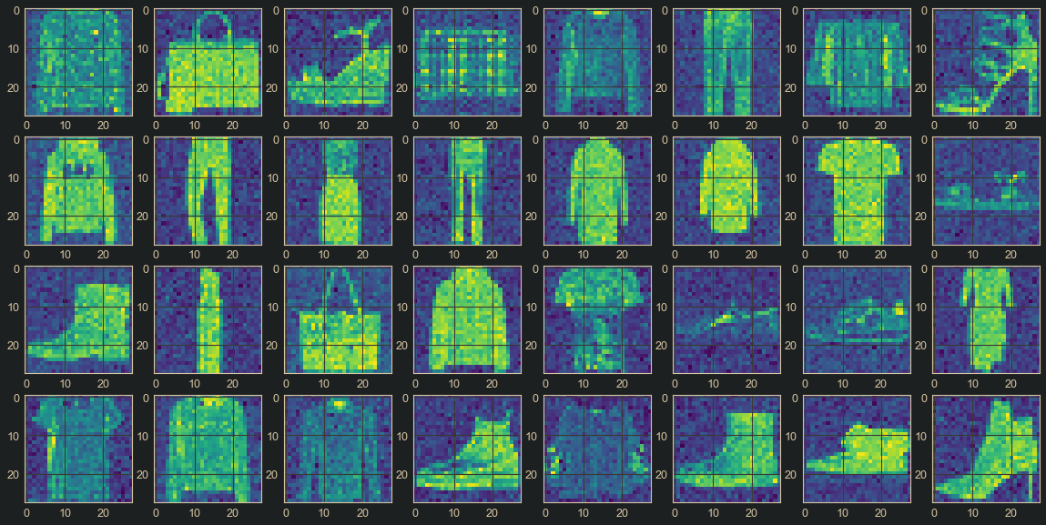
Figure 5. : Corrupted Image Batch

Next, we need to design our model architecture. Remember, as an autoencoder, our DAE must comprise an Encoder and a Decoder. They are built respectively via Sequential API:

def get_encoder(shape = (28, 28, 1)):

    ''' Generate Encoder model. '''
    
    encoder = Sequential()

    encoder.add(layers.Input(shape = shape))
    
    encoder.add(layers.Conv2D(filters = 32, kernel_size = (3, 3), padding = 'same'))
    encoder.add(layers.BatchNormalization())
    encoder.add(layers.LeakyReLU(0.2))
    encoder.add(layers.MaxPool2D())

    encoder.add(layers.Conv2D(filters = 64, kernel_size = (3, 3), padding = 'valid'))
    encoder.add(layers.BatchNormalization())
    encoder.add(layers.LeakyReLU(0.2))
    encoder.add(layers.MaxPool2D())

    encoder.add(layers.Conv2D(filters = 128, kernel_size = (3, 3), padding = 'valid'))
    encoder.add(layers.BatchNormalization())
    encoder.add(layers.LeakyReLU(0.2))
    
    encoder.add(layers.Reshape((tf.math.reduce_prod(encoder.output.shape[1:]).numpy(),)))
    
    return encoder

def get_decoder(shape_source = encoder):
    
    ''' Generate Decoder model. '''
    
    decoder = Sequential()

    decoder.add(layers.Input(shape = tuple(shape_source.output.shape[1:])))
    decoder.add(layers.Reshape(tuple(shape_source.layers[-2].output.shape[1:])))

    decoder.add(layers.Conv2DTranspose(filters = 64, kernel_size = (3, 3), padding = 'valid'))
    decoder.add(layers.BatchNormalization())
    decoder.add(layers.LeakyReLU(0.2))
    decoder.add(layers.UpSampling2D())

    decoder.add(layers.Conv2DTranspose(filters = 32, kernel_size = (3, 3), padding = 'same'))
    decoder.add(layers.BatchNormalization())
    decoder.add(layers.LeakyReLU(0.2))
    decoder.add(layers.UpSampling2D())

    decoder.add(layers.Conv2DTranspose(filters = 1, kernel_size = (3, 3), padding = 'valid'))
    decoder.add(layers.BatchNormalization())
    decoder.add(layers.LeakyReLU(0.2))

    decoder.add(layers.Conv2DTranspose(filters = 1, kernel_size = (3, 3), padding = 'valid', activation = 'sigmoid'))
    
    return decoder

The description for the encoder and decoder are shown respectively:

Input:

encoder.summary()

Output:

Model: "sequential"
_________________________________________________________________
 Layer (type)                Output Shape              Param #   
=================================================================
 conv2d (Conv2D)             (None, 28, 28, 32)        320       
                                                                 
 batch_normalization (BatchN  (None, 28, 28, 32)       128       
 ormalization)                                                   
                                                                 
 leaky_re_lu (LeakyReLU)     (None, 28, 28, 32)        0         
                                                                 
 max_pooling2d (MaxPooling2D  (None, 14, 14, 32)       0         
 )                                                               
                                                                 
 conv2d_1 (Conv2D)           (None, 12, 12, 64)        18496     
                                                                 
 batch_normalization_1 (Batc  (None, 12, 12, 64)       256       
 hNormalization)                                                 
                                                                 
 leaky_re_lu_1 (LeakyReLU)   (None, 12, 12, 64)        0         
                                                                 
 max_pooling2d_1 (MaxPooling  (None, 6, 6, 64)         0         
 2D)                                                             
                                                                 
 conv2d_2 (Conv2D)           (None, 4, 4, 128)         73856     
                                                                 
 batch_normalization_2 (Batc  (None, 4, 4, 128)        512       
 hNormalization)                                                 
                                                                 
 leaky_re_lu_2 (LeakyReLU)   (None, 4, 4, 128)         0         
                                                                 
 reshape (Reshape)           (None, 2048)              0         
                                                                 
=================================================================
Total params: 93,568
Trainable params: 93,120
Non-trainable params: 448
_________________________________________________________________

Input:

decoder.summary()

Output:

Model: "sequential_1"
_________________________________________________________________
 Layer (type)                Output Shape              Param #   
=================================================================
 reshape_1 (Reshape)         (None, 4, 4, 128)         0         
                                                                 
 conv2d_transpose (Conv2DTra  (None, 6, 6, 64)         73792     
 nspose)                                                         
                                                                 
 batch_normalization_3 (Batc  (None, 6, 6, 64)         256       
 hNormalization)                                                 
                                                                 
 leaky_re_lu_3 (LeakyReLU)   (None, 6, 6, 64)          0         
                                                                 
 up_sampling2d (UpSampling2D  (None, 12, 12, 64)       0         
 )                                                               
                                                                 
 conv2d_transpose_1 (Conv2DT  (None, 12, 12, 32)       18464     
 ranspose)                                                       
                                                                 
 batch_normalization_4 (Batc  (None, 12, 12, 32)       128       
 hNormalization)                                                 
                                                                 
 leaky_re_lu_4 (LeakyReLU)   (None, 12, 12, 32)        0         
                                                                 
 up_sampling2d_1 (UpSampling  (None, 24, 24, 32)       0         
 2D)                                                             
                                                                 
 conv2d_transpose_2 (Conv2DT  (None, 26, 26, 1)        289       
 ranspose)                                                       
                                                                 
 batch_normalization_5 (Batc  (None, 26, 26, 1)        4         
 hNormalization)                                                 
                                                                 
 leaky_re_lu_5 (LeakyReLU)   (None, 26, 26, 1)         0         
                                                                 
 conv2d_transpose_3 (Conv2DT  (None, 28, 28, 1)        10        
 ranspose)                                                       
                                                                 
=================================================================
Total params: 92,943
Trainable params: 92,749
Non-trainable params: 194
_________________________________________________________________

Now, we can construct the final DAE model. This will be done via the Functional API in Tensorflow:

### Finalize the model via Functional API

encoder = get_encoder(shape = (28, 28, 1))
decoder = get_decoder(shape_source = encoder)

final_output = decoder(encoder.output)

DAE = Model(encoder.input, final_output)

We can get a summary of our composite model as shown:

Input:

### Denoising Autoencoder info
DAE.summary()

Output:

Model: "model"
_________________________________________________________________
 Layer (type)                Output Shape              Param #   
=================================================================
 input_3 (InputLayer)        [(None, 28, 28, 1)]       0         
                                                                 
 conv2d_3 (Conv2D)           (None, 28, 28, 32)        320       
                                                                 
 batch_normalization_6 (Batc  (None, 28, 28, 32)       128       
 hNormalization)                                                 
                                                                 
 leaky_re_lu_6 (LeakyReLU)   (None, 28, 28, 32)        0         
                                                                 
 max_pooling2d_2 (MaxPooling  (None, 14, 14, 32)       0         
 2D)                                                             
                                                                 
 conv2d_4 (Conv2D)           (None, 12, 12, 64)        18496     
                                                                 
 batch_normalization_7 (Batc  (None, 12, 12, 64)       256       
 hNormalization)                                                 
                                                                 
 leaky_re_lu_7 (LeakyReLU)   (None, 12, 12, 64)        0         
                                                                 
 max_pooling2d_3 (MaxPooling  (None, 6, 6, 64)         0         
 2D)                                                             
                                                                 
 conv2d_5 (Conv2D)           (None, 4, 4, 128)         73856     
                                                                 
 batch_normalization_8 (Batc  (None, 4, 4, 128)        512       
 hNormalization)                                                 
                                                                 
 leaky_re_lu_8 (LeakyReLU)   (None, 4, 4, 128)         0         
                                                                 
 reshape_2 (Reshape)         (None, 2048)              0         
                                                                 
 sequential_3 (Sequential)   (None, 28, 28, 1)         92943     
                                                                 
=================================================================
Total params: 186,511
Trainable params: 185,869
Non-trainable params: 642
_________________________________________________________________

We are almost at the finish line! All we need now are our hyperparameters:

• Learning rate (3e-6),
• Optimizer (Adam),
• Number of epochs (20), and
• Objective function (mean squared error)

### Instantiate training objects and hyperparameters
epochs = 20
criterion = tf.losses.MeanSquaredError()
opt = optimizers.Adam(learning_rate = 3e-6, beta_1 = 0.99, beta_2 = 0.999)

With all we need in hand, we can begin to train our model. The most popular way most people use is via the well-known fit method:

DAE.compile(criterion
DAE.fit(data, epochs, ...)

However, for educational purposes, we will design our own training loop from scratch. It should be noted that irrespective of the framework, the training loop follows a basic pipeline. In other words, the training process is largely the same even if we were to use a different framwork, say mxnet. Since we are not absracting away the details (as the fit method would allow us do), we can be said to be building a low-level training loop:

1. Take a data batch.
2. Pass the batch into the model.
3. Get the model outputs.
4. Compare the outputs to the ground truth i.e. labels. This gives the loss.
5. Obtain the gradient of the loss w.r.t. to the model parameters.
6. Backpropagate the loss through the model and apply parameter updates.
7. Return to Step 1.

These steps will guide our training process. With these steps in mind, we design the training loop:

### Training loop
for epoch in range(1, epochs + 1):
    iteration = 0 ### Number of iterations per epoch of training
    
    for batch in X_train: ### Inner loop for the data batchs
        ### Corrupt data batch and clip
        inputs = batch + tf.random.normal(mean = 0., stddev = 0.1, shape = batch.shape)
        inputs = tf.clip_by_value(inputs, 0., 1.)
        
        ### Compute loss
        with tf.GradientTape() as tape:
            outputs = DAE(inputs)
            loss = criterion(batch, outputs)
    
        ### Obtain gradients w.r.t loss
        grads = tape.gradient(loss, DAE.trainable_variables)

        ### Apply the gradients to model parameters
        opt.apply_gradients(zip(grads, DAE.trainable_variables))

        ### Keep track of iterations per epoch
        iteration += 1

        ### Regularly visualize denoised images
        if not (iteration % 25) or iteration == len(X_train):
            print(f'\nEpoch {epoch}/{epochs}; Iteration {iteration}:\n\tLoss: {loss.numpy():.4f}', end = '\n')
            visualize(outputs)

After training for 20 epochs, the final result obtained is visualized:

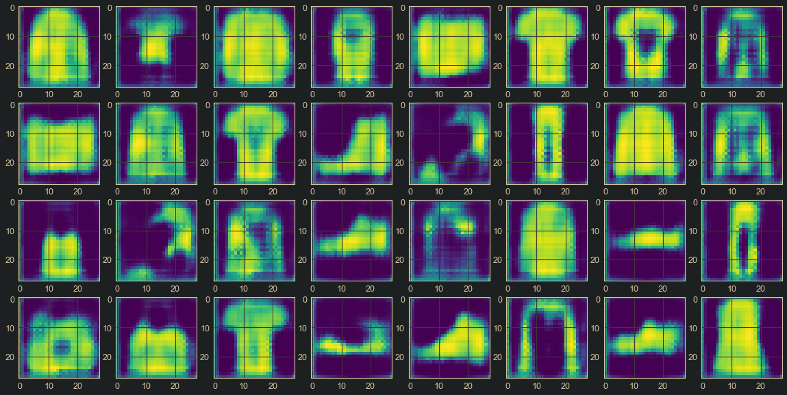
Figure 6. : Final Reconstructed Image

As can be seen from the image above, the quality is not so good, but the DAE is defnitely learning something. Improving performance is left as an exercise to the reader. Hints on how to do so include:

• Train for longer epochs.
• Reduce/increase the batch size.
• Attempt parameter norms.
• Try out different optimizers and learning rates.

---

Resources

Below are a few videos which might help gain more clarification:

Conclusion

With this article at OpenGenus, you must have the complete idea of Denoising Autoencoders (DAEs).