
In this article, we will be learning about different Classification tree methods such as C4.5, CHAID and much more along with some key similarities and differences between them. An implementation in Python is also explained.
Contents
- Introduction to Decision Trees
- Common Distinguishing Features
- Different Decision Tree Classification Algorithms
- Implementation
- Conclusion
Introduction to Decision Trees
A decision tree is a type of supervised machine learning algorithm that is used to categorize or make predictions based on a set of questions that are asked.
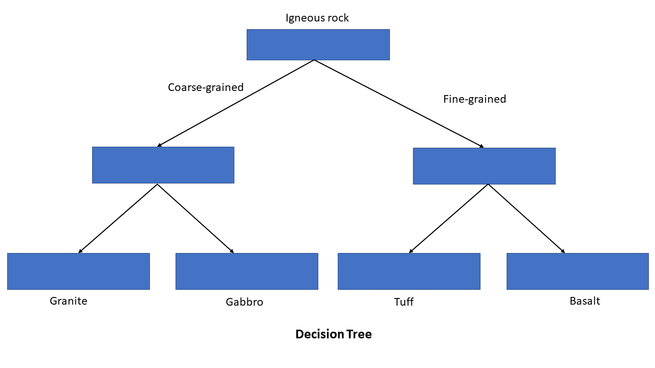
Above is an example of a simple decision tree. It asks a series of questions that lead to the final decision.
There are a variety of algorithms that can be used to create decision trees for classification (classifying between distinct classes) or regression (outputting a continuous numerical value).
Common Distinguishing Features of Different Methods
Split Selection Criteria
At every step, decision trees split on the feature that leads to the optimal result. But, how do decision trees determine the best feature? There are various measures/algorithms for this, and different decision tree algorithms use different techniques. Techniques may have selection bias, which is the tendency to select a specific type of feature over another.
Below are some common split selection techniques:
Entropy
Entropy essentially measures the uncertainty of the target based on a feature. Higher entropy means more uncertainty, and the goal of trees that use entropy is to minimize it in order to make the most accurate predictions. Entropy is measured between 0 and 1, and values closer to 0 correlate with lower degrees of uncertainity (i.e. higher degrees of certainty).
Information Gain
Information Gain calculates the reduction in entropy, and this measures how well a given feature separates the target classes. Like the name suggests, Information Gain measures how much certainty of the target variable is gained by having knowledge of a certain feature.
The feature with the highest Information Gain is selected as the best one. After selecting an optimal feature, the ID3 algorithm splits the dataset into subsets, and this process is repeated on the subsets using the remaining features (using recursion). This recursion stops when there are no more attributes to be selected or every element in the subset belongs to the same class. Throughout this process, the decision tree is constructed using nodes that represent each feature the data was split on.
Information Gain Ratio
Information Gain Ratio improves on some shortcomings of Information Gain. If the Entropy of two features is the same, Information Gain may favor the feature with a higher number of distinct values. However, features with less distinct values are usually better at generalizing to unseen samples.
For example, if we want to determine some specific information about an individual, some kind of identification number would have a high information gain because it uniquely identifies individuals, but it will not generalize well when tested on unseen samples of data. Therefore, it is not an optimal feature.
Information Gain Ratio helps solve this problem by favoring features/attributes with a lower number of distinct values.
Gini Impurity
The Gini Impurity of a dataset is a number between 0 and 0.5, which indicates the likelihood of unseen data being misclassified if it were given a random class label according to the class distribution in the dataset.
When training a decision tree, the best split is chosen by minimizing the Gini Impurity.
Chi-square test of independence
The Chi-square test of independence checks whether two variables are likely to be related or not. This test returns the degree of independence between the two variables. The feature that has the least degree of independence is selected as the feature to split on.
Early Stopping vs Post-Pruning
Two of the main techniques used for reducing tree size (to prevent overfitting and underfitting) are early-stopping (pre-pruning) and post-pruning.
Pruning is a reduces the size of decision trees by removing branches that are non-critical and redundant to classify instances.
Post-pruning is used after the entire decision tree is constructed. This technique is used when the decision tree has a very large depth and is likely to overfit on the training data.
Early Stopping (Pre-Pruning), on the other hand, involves stopping the tree before it has completed.
Trade-offs between the two: Early stopping is usually faster than post-pruning, but post-pruning usually leads to a more accurate tree. The reason post-pruning is usually more accurate is that early stopping is a greedy algorithm, so it's possible that it ignores splits that have importaqaant splits that follow.
Classification Methods
For classification, we will be discussing the following algorithms:
- ID3
- C4.5
- CART
- GUIDE
- FACT
- QUEST
- CRUISE
- CHAID
ID3
ID3 stands for Iterative Dichotomiser 3. This algorithm repeatedly divides features into several subgroups. It uses a top-down greedy approach, which means that it constructs the tree from the top, and at each step, it selects the best feature to split the dataset on.
- ID3 uses Information Gain (and thus Entropy as well) to determine the best feature to split on.
- ID3 may have a selection bias towards features with a greater number of distinct values.
One limitation of the ID3 algorithm is that it is used on categorical data (data that has a discrete number of possible values). This is because if the values of a feature are continuous, then there are many places to split the data on this attribute, and finding the best value to split on may be time-consuming.
C4.5
The C4.5 algorithm is a successor of ID3. The most significant difference between C4.5 and ID3 is that C4.5 efficiently allows for continuous features by partitioning numerical values into distinct intervals.
- Instead of Information Gain, C4.5 uses Information Gain Ratio to determine the best feature to split on.
- C4.5 uses post-pruning after growing an overly large tree.
- C4.5 has a bias towards features with a lesser number of distinct values.
CART (Classification and Regression Tree)
CART, similarly to C4.5, supports both categorical and numerical data. However, CART differs from C4.5 in the way that it also supports regression.
One major difference between CART, ID3, and C4.5 is the feature selection criteria. While ID3 and C4.5 use Entropy/Information Gain/Information Gain Ratio, CART uses Gini Impurity. Additionally, CART constructs a binary tree, which means that every node has exactly two children, unlike the other algorithms we have discussed, which don't necessarily have two child nodes per parent.
- When training a CART decision tree, the best split is chosen by minimizing the Gini Impurity.
- CART uses post-pruning after growing an overly large tree.
FACT, QUEST, CRUISE and GUIDE
The FACT algorithm was the first to be implemented out of these four algorithms, and the other three algorithms are progressions of FACT.
FACT:
- Uses the ANOVA F-test and applies Linear Discriminant Analysis (LDA) to the feature that has the most significant ANOVA F-test.
- There is a selection bias toward categorical variables, because LDA is used twice on each categorical variable.
QUEST
- Corrects the selection bias present in the FACT algorithm by using chi-square tests for categorical variables instead of F-tests.
CRUISE
- Uses chi-square tests.
- Discretizes each ordered variable into a categorical variable.
- Splits each node into several branches, with one for each class.
- Free of selection bias
GUIDE
- The main difference between GUIDE and its predecessors is how it handles missing values - while CRUISE and QUEST use imputation to deal with missing values, GUIDE assigns a special category for them.
- Free of selection bias
Chi-square automatic interaction detection (CHAID)
- CHAID uses chi-square test of independence for feature selection.
- There is a selection bias toward variables with few distinct values.
Additionally, each ordered variable is split into several intervals, with one child node being assigned to each of those intervals. Each feature that is unordered has one child node assigned to each distinct value of that feature.
Implementation
A decision tree can be implemented fairly quickly in Python, using the scikit-Learn library. According to the documentation, "scikit-learn uses an optimized version of the CART algorithm; however, scikit-learn implementation does not support categorical variables for now." (There are several techniques to deal with categorical variables.)
In order to run the following code, you will need to have installed scikit-learn using the following command:
pip install scikit-learn
The first step is to import the tree module from scikit-learn, using the following code:
from sklearn import tree
In this article, we won't import an existing dataset, but we can pass in our own data in a 2D array format.
Below is the data we will be using, in a tabular format.
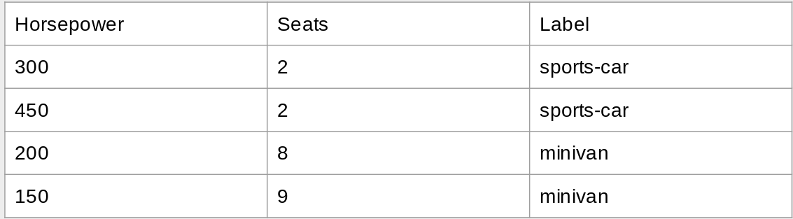
We can represent the features (independent variables) using a 2D list. The labels (correct class) are stored in a 1D list, as shown below:
features = [[300, 2], [450, 2], [200, 8], [150, 9]]
labels = ["sports-car", "sports-car", "minivan", "minivan"]
Note: the order matters! Each element in labels should correspond with the features at the same index. For example, the third sample's label is "minivan". The features [200, 8] correspond with that sample.
Next, we create our model and train it using the fit() function.
model = tree.DecisionTreeClassifier()
model.fit(features, labels)
We can test our model on unseen data as shown below:
print(model.predict([[500, 2], [100, 10], [150, 6]]))
Output:['sports-car' 'minivan' 'minivan']
We can see the steps the tree takes to predict on unseen data by plotting the model. Scikit-learn offers a very easy-to-use function plot_tree() to do this. Matplotlib (pip install matplotlib) must be installed in order to run the following code.
import matplotlib.pyplot as plt

fig = plt.figure(figsize=(25,20))
_ = tree.plot_tree(model,
                   feature_names=["Horsepower", "Seats"],
                   class_names=["Sports car", "Minivan"],
                   filled=True)
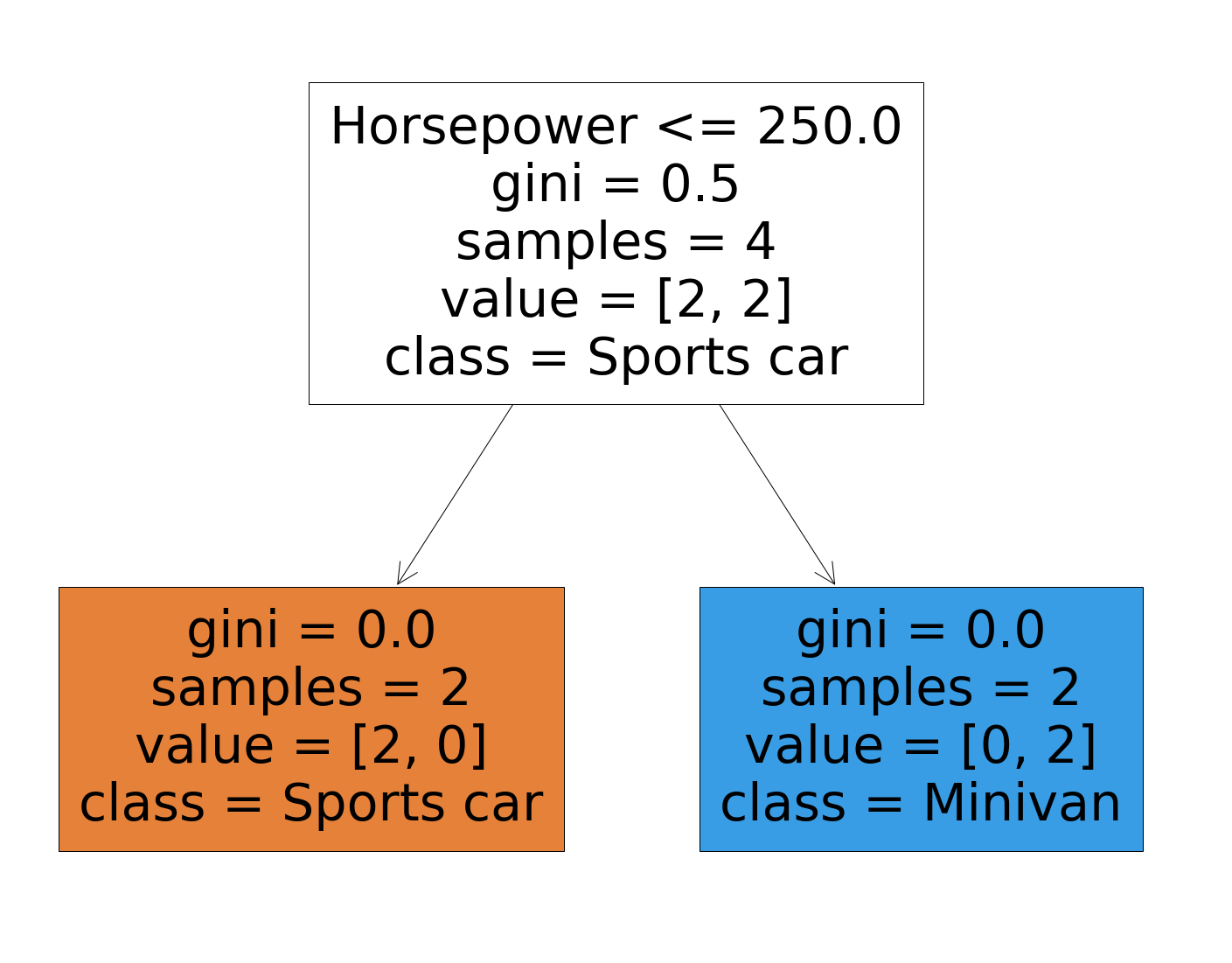
As shown in the image, the tree only required one split (Horsepower) to reach the final decision. The feature Horsepower led to a perfect separation, as evidenced by a Gini Impurity score of 0.
Conclusion
In this article, we learned about different types of decision trees and how they are constructed, as well as how to implement one in Python.
Thanks for reading!