Different Self Balancing Binary Trees

A self-balancing binary tree is any tree that automatically keeps its height small in the face of arbitrary insertions and deletions on the tree. The height is usually maintained in the order of log n so that all operations performed on that tree take O(log n) time on an average. Now let us look at the most widely used self balancing binary trees, their complexities and their use cases. The various self balancing binary search trees are:

1. 2-3 tree
2. Red-Black Tree
3. AVL tree
4. B tree
5. AA tree
6. Scapegoat Tree
7. Splay tree
8. Treap
9. Weight Balanced trees

1. 2-3 Tree

A 2-3 tree is a self-balancing binary tree data structure where each node in the tree has either:

• 2 children and 1 data element.
• 3 children and 2 data elements.
• Leaf nodes are at the same level and have no children but have either 1 or 2 data elements.

Learn more about 2-3 Tree in detail

An example of a 2-3 tree is shown below.

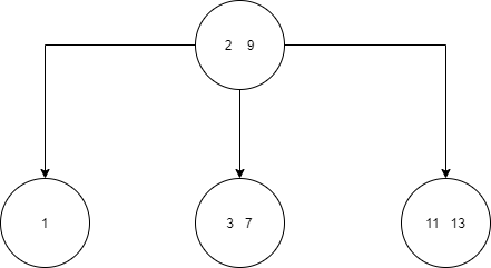
You can see from the above tree that it satisfies all the rules mentioned above.
Time Complexity in Big O notation: The time complexity for average and worst case is the same for a 2-3 tree i.e.

• Space - O(n)
• Search - O(log n)
• Insert - O(log n)
• Delete - O(log n)

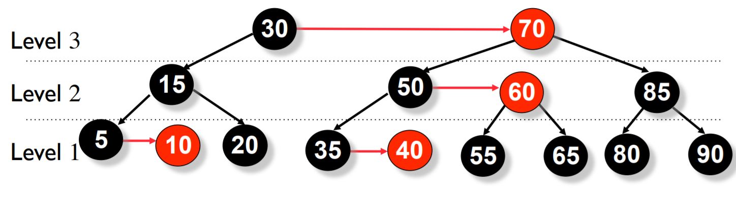
2. Red-Black Tree

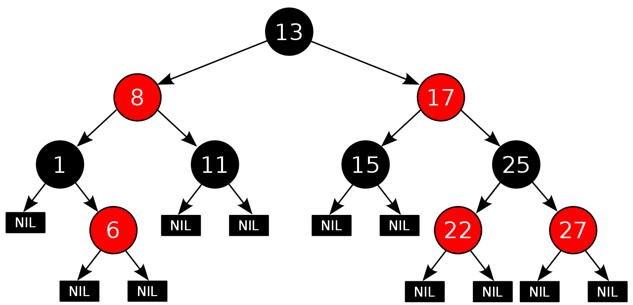
A Red-Black tree is another self balancing binary search tree. Here each node stores an extra bit which represents the color which is used to ensure that the tree remains balanced during the insertion and deletion operations. Here every node has the following rules in addition to that imposed by a binary search tree:

• Every node is either colored red or black.
• Root of the tree is always black.
• All leaves i.e NIL are always black.
• There are no two adjacent red nodes i.e. a red node cannot have a red child or a red parent.
• Every path from a node to any of its descendant NIL node has the same number of black nodes.

Learn more about Red Black tree in detail

Below is an example of a red-black tree.

Time Complexity in Big O notation: The time complexity for average and worst case is the same for a red-black tree i.e.

• Space - O(n)
• Search - O(log n)
• Insert - O(log n)
• Delete - O(log n)

3. AVL Tree

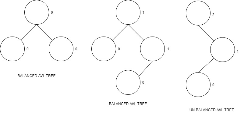
AVL tree is a type of self-balancing binary search tree where the difference between heights of the left and right subtrees cannot be more than one for all nodes in the tree. This is called the Balance Factor and is defined to be:
BalanceFactor(node) = Height(RightSubTree(node)) - Height(LeftSubTree(node)) which is an integer from the set {-1, 0, 1} if it is an AVL tree.

You can read more about AVL trees in the article at OpenGenus IQ here.
Time Complexity in Big O notation: The time complexity for an AVL tree is as shown below

• Space - O(n)
• Search - O(log n)
• Insert - O(log n)
• Delete - O(log n)

4. B-tree

A B-Tree is a type of self balancing binary search tree which generalizes the binary search tree, allowing for nodes with more than 2 children.
According to Knuth's definition, a B-tree of order m is a tree which satisfies the following properties:

1. Every node has at most m children.
2. Every non-leaf node (except root) has at least ⌈m/2⌉ child nodes.
3. The root has at least two children if it is not a leaf node.
4. A non-leaf node with k children contains k − 1 keys.
5. All leaves appear in the same level and carry no information.

Below is an example of a B-Tree.

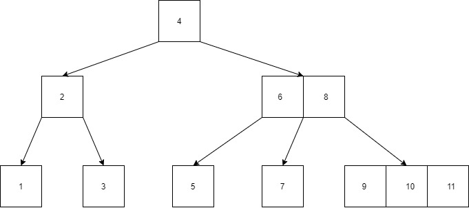
A B-Tree of order 3 is a 2-3 Tree.
Time Complexity in Big O notation: The time complexity for a B-Tree (Average and Worst Case) shown below

• Space - O(n)
• Search - O(log n)
• Insert - O(log n)
• Delete - O(log n)

Applications of B-Trees:

• Well suited for storage systems that read and write relatively large block of data.
• Used in databases and file systems.

5. AA Tree

Unlike in red-black trees, red nodes on an AA tree can only be added as a right sub-child i.e. no red node can be a left sub-child. The following five invariants hold for AA trees:

1. The level of every leaf node is one.
2. The level of every left child is exactly one less than that of its parent.
3. The level of every right child is equal to or one less than that of its parent.
4. The level of every right grandchild is strictly less than that of its grandparent.
5. Every node of level greater than one, has two children.

Below is an example of an AA tree.

It guarantees fast operations in Θ(log n) time, and the implementation code is perhaps the shortest among all the balanced trees.
For a complete understanding of AA-Trees, you can read another article I wrote here.

6. Scapegoat Tree

A scapegoat tree is a self-balancing variant of the binary search tree. Unlike other self balancing trees, scapegoat tree does not require any extra storage per node of the tree. The low overhead and easy implementation makes the scapegoat tree a very attractive option as a self balancing binary search tree.
The balancing idea is to make sure that nodes are α (alpha) size balanced. What this means is that the sizes of left and right subtrees are at most α times (size of node) i.e. α * (size of node). This concept is based on the fact that if a node is α weight balanced, it is also height balanced with height less than log_(1/α)⁡size + 1.
Time Complexity in Big O notation (Average Case) : The time complexity for a Scapegoat tree for average case is as shown below

• Space - O(n)
• Search - O(log n)
• Insert - O(log n)
• Delete - O(log n)

Time Complexity in Big O notation (Worst Case) : The time complexity for a Scapegoat tree for worst case is as shown below

• Space - O(n)
• Search - O(log n)
• Insert - amortized O(log n)
• Delete - amortized O(log n)

7. Splay tree

A splay tree is a self-balancing binary search tree with the additional property that recently accessed elements are quick to access again. All normal operations on a binary tree are combined with one basic operation called splaying. Splaying of the tree for a certain element rearranges the tree so that the element is placed at the root of the tree.
For example, when you perform a standard binary search for an element in question, and then use the tree rotations in a specific order such that this element is now placed as the root. We could also make use of a top-down algorithm to combine the search and the reorganization into a single phase.
Splaying depends on three different factors when we try to access an element called x:

1. whether x is the left or right child of its parent node p
2. whether p is the root or not, and if not
3. wheter p is the left or right child of its parent g (the grandparent of x)

Based on this, we have three different types of operations:

1. Zig: This step is done when p is the root.
   
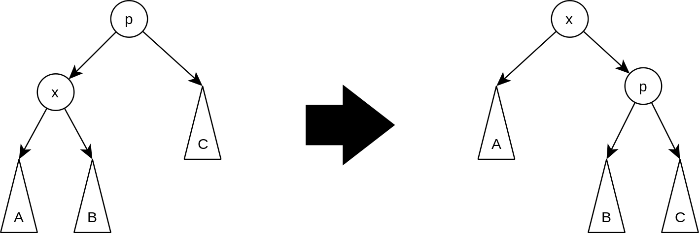
2. Zig-Zig: This step is done when p is not the root and x and p are either both right children or are both left children.
   
3. Zig-Zag: This is done when p is not the root and x is a right child and p is a left child or vice versa.
   

Time Complexity in Big O notation (Average Case) : The time complexity for the search, insert and delete operations in average case is O(log n).
Time Complexity in Big O notation (Worst Case) : The time complexity for a Splay tree for worst case is as shown below

• Space - O(n)
• Search - amortized O(log n)
• Insert - amortized O(log n)
• Delete - amortized O(log n)

8. Treap

Treap is a data structure that combines both a binary tree and a binary heap but it does not guarantee to have a height of O(log n). The concept is to use randomization and binary heap property to maintain balance with high probability.
Every node of a treap contains 2 values:

1. KEY which follows standard binary search tree ordering.
2. PRIORITY which is a randomly assigned value that follows max-heap property.

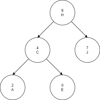
The above example is a treap with alphabetic key and numeric max heap order.
Treaps support the following basic operations:

1. To search for a given key value, apply a standard binary search algorithm in a binary search tree, ignoring the priorities.
2. To insert a new key x into the treap, generate a random priority y for x. Binary search for x in the tree, and create a new node at the leaf position where the binary search determines a node for x should exist. Then, as long as x is not the root of the tree and has a larger priority number than its parent z, perform a tree rotation that reverses the parent-child relation between x and z.
3. To delete a node x from the treap, if x is a leaf of the tree, simply remove it. If x has a single child z, remove x from the tree and make z be the child of the parent of x (or make z the root of the tree if x had no parent). Finally, if x has two children, swap its position in the tree with the position of its immediate successor z in the sorted order, resulting in one of the previous cases. In this final case, the swap may violate the heap-ordering property for z, so additional rotations may needed to be performed to restore this property.

Time Complexity in Big O notation (Average Case) : The time complexity for a Treap for average case is as shown below

• Space - O(n)
• Search - O(log n)
• Insert - O(log n)
• Delete - O(log n)

Time Complexity in Big O notation (Worst Case) : The time complexity for a Treap for worst case is as shown below

• Space - O(n)
• Search - O(n)
• Insert - O(n)
• Delete - O(n)

9. Weight Balanced trees

Weight-balanced trees are binary search trees, which can be used to implement finite sets and finite maps. Although other balanced binary search trees such as AVL trees and red-black trees use height of subtrees for balancing, the balance of WBTs is based on the sizes of the subtrees below each node. The size of a tree is the number of associations that it contains. Weight-balanced binary trees are balanced to keep the sizes of the subtrees of each node within a constant factor of each other. This ensures logarithmic times for single-path operations (like lookup and insertion). A weight-balanced tree takes space that is proportional to the number of associations in the tree.
A node of a WBT has the fields

• key of any ordered type
• value (optional) for mappings
• left and right pointer to nodes
• size of integer type

Conclusion

Self-balancing BSTs are flexible data structures, in that it's easy to extend them to efficiently record additional information or perform new operations. For example, one can record the number of nodes in each subtree having a certain property, allowing one to count the number of nodes in a certain key range with that property in O(log n) time. These extensions can be used, for example, to optimize database queries or other list-processing algorithms.

With this article at OpenGenus, the idea of Different Self Balancing Binary Trees must be clear. Enjoy.