Open-Source Internship opportunity by OpenGenus for programmers. Apply now.
We have explored a technique to Differentiate fake faces using simple Machine Learning (ML) and computer vision. We have used Large-scale CelebFaces Attributes dataset.
Introduction
In the past, photographs and images were available as analog images, impervious to any modifications. However, this has changed as increase in technology has made way for the digital era, where even our photographs are now a sequence of 0s and 1s. With increased sophistication of smartphones and rise in social network growth, the internet is flooded with tremendous amount of digital content. With this amount of data available there came the existence of techniques that could alter the image data. Digital manipulation of images and videos are a matter of concern today. These images and videos are popularly known as "Deepfakes". The terminology was first originated in 2017 and uses deep learning models to swap the face of a person to another. This technique could lead to creation of fake content including fake news, hoaxes, and financial fraud.
Generally, the number and authenticity of facial controls have been restricted by the absence of modern altering instruments, the area aptitude required, and the complex and tedious cycle included. For instance, an early work in this theme had the option to change the lip movement of an individual talking utilizing an alternate sound track, by making associations between the hints of the sound track and the state of the subject's face. Be that as it may, from these early works forward-thinking, numerous things have quickly advanced in the most recent years. These days, it is getting progressively simple to consequently orchestrate non-existent faces or control a genuine face of one individual in a picture/video, on account of: i) the openness to enormous scope public information, and ii) the development of profound learning procedures that dispense with numerous manuals altering steps, for example, Variable Autoencoders (VAE) and Generative Adversarial Networks (GAN). This has opened the way for developers to create portable applications like FaceApp and ZAO. These applications have opened the entryway to anybody to make fake pictures and recordings, with no experience required.
What Methodology is used?
Current deepfake detection techniques rely on high amount of labelled data and the use of adversarial networks and autoencoders which take time to build and train.
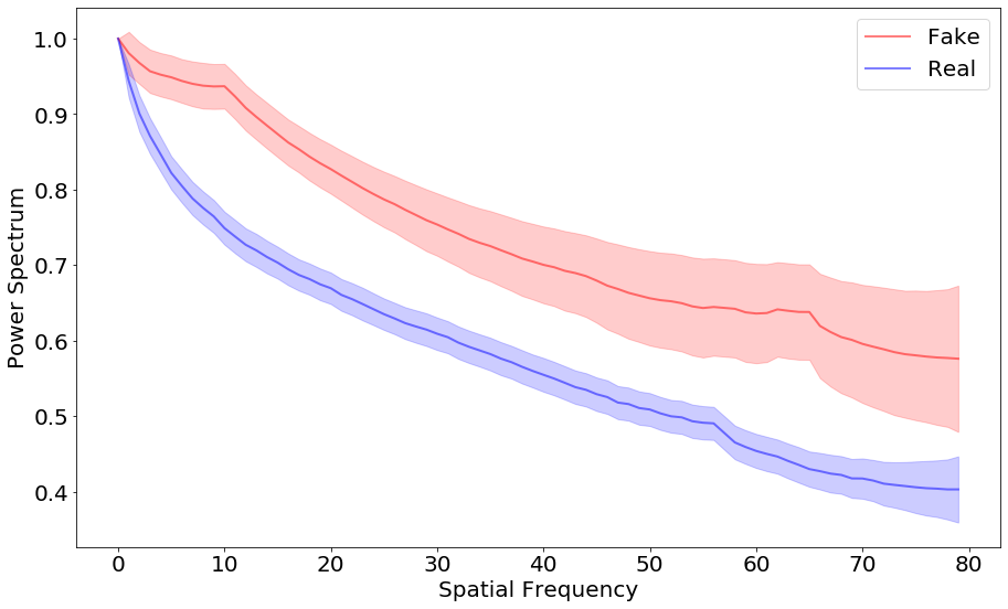
Popular Generative Adversarial Networks such as WGAN-GP, DRA-GAN, DCGAN, and LSGAN relies on convolutional up-sampling methods like transpose-convolution and up-convolution. These methods when applied to images alter their spectral distribution which makes them susceptible to detect themselves as fake.
To put it in simpler words, when popular deep learning models are applied to images in order to alter them, they would look more or less same to you, but if we transform the image and look it in the frequency domain and compare the "before" image (not modified) and "after" image (modified), we will see that the spectrum has been changed.
How to view images in the frequency domain?
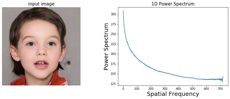
We use Discrete Fourier Transform to convert the image in the frequenct domain. Discrete Fourier Transform, or DFT is a mathematical technique primarily used in signal processing to find the spectrum of a finite duration signal. The technique breaks down a discrete signal into its sine and cosine components. The input image, present in its spatial domain is converted to the Fourier or frequency domain. Each point in the frequency domain represents a particular frequency in the spatial domain.
It is to be noted that the number of pixels in the spatial domain image corresponds to the number of frequencies, thus making the image in the spatial and fourier domain of the same size. This means that the information is presented in a new domain but has the same dimensionality. To convert and represent this 2-D information into 1-D, we apply azimuthal average to our power spectrum. to put it in simpler terms, this step is a compression technique that gathers similar frequency components and averages them into a feature vector. This reduces the features but does not affect the performance nor it loses any relevant information.
Analysis done. How to classify?
With our information successfully analysed and transformed into our desired way, the next step involves classification. Classification will enable us to differentiate the images between real and fake. There are many algorithms that you can use in order to classify but in this one, we will be using Support Vector Machines mainly because of its popularity on non-linear data classification.
By now, you guys would be wondering: On which data is this done? Well, there are many datasets available on the internet but there is no public dataset big enough that encapsulates both real as well as fake faces. But, there are individual datasets that you can use to run this model.
In this project, Large-scale CelebFaces Attributes dataset, also known as CelebA dataset is used. This image set has over 200K celebrity faces in 40 different annotations. There is also the FlickrFaces-HQ dataset which has high resolution images that is primarily used as a benchmark for GAN networks. These datasets provide images for the 'real' image class. For the 'fake' image class, there is the 100k faces project which contains over 70K images generated using AI. Also, there is a website by the name of thispersondoesnotexist which gives users an AI-generated image every time the page is reloaded. To get images from this site, you would need to know the basics of webscrapping. There are plenty of tutorials online that can tell you to get anything you want from the internet in just 10 minutes.
Tools required
This project is done in Python in Jupyter Notebook. Modules used are openCV, numpy, matplotlib and scikit-learn.
To calculate the azimuthal average, visit this link to use the radialProfile script. This will save you some time.
Code
1. Visualization of image in frequency domain
import cv2
import numpy as np
from matplotlib import pyplot as plt
import matplotlib.image as mpimg
import radialProfile

epsilon = 1e-8
filename = '100KFake_10K/1.jpg'

img = cv2.imread(filename,0)
img_color = mpimg.imread(filename)
# Calculate FFT
f = np.fft.fft2(img)
fshift = np.fft.fftshift(f)
fshift += epsilon
magnitude_spectrum = 20*np.log(np.abs(fshift))
# Calculate the azimuthally averaged 1D power spectrum
psd1D = radialProfile.azimuthalAverage(magnitude_spectrum)

#Visualization
fig = plt.figure(figsize=(15,5))
ax = fig.add_subplot(121)
plt.axis('off')
ax2 = fig.add_subplot(122)
ax.set_title('input image',size=15)
ax2.set_title('1D Power Spectrum',size=15)
plt.xlabel('Spatial Frequency', fontsize=20)
plt.ylabel('Power Spectrum', fontsize=20)
ax.imshow(img_color)
ax2.plot(psd1D)
plt.show()

2. Classification using celebA dataset and fake celebA dataset
import cv2
import numpy as np
import os
import radialProfile
import glob
from matplotlib import pyplot as plt
import pickle
from scipy.interpolate import griddata

data= {}
epsilon = 1e-8
N = 80
y = []
error = []

number_iter = 1000

psd1D_total = np.zeros([number_iter, N])
label_total = np.zeros([number_iter])
psd1D_org_mean = np.zeros(N)
psd1D_org_std = np.zeros(N)


cont = 0

#fake data
rootdir = 'dataset_celebA/'

for filename in glob.glob(rootdir+"*.jpg"):
    img = cv2.imread(filename,0)

    f = np.fft.fft2(img)
    fshift = np.fft.fftshift(f)
    fshift += epsilon

    magnitude_spectrum = 20*np.log(np.abs(fshift))
    psd1D = radialProfile.azimuthalAverage(magnitude_spectrum)

    # Calculate the azimuthally averaged 1D power spectrum
    points = np.linspace(0,N,num=psd1D.size) # coordinates of a
    xi = np.linspace(0,N,num=N) # coordinates for interpolation

    interpolated = griddata(points,psd1D,xi,method='cubic')
    interpolated /= interpolated[0]

    psd1D_total[cont,:] = interpolated
    label_total[cont] = 1
    cont+=1

    if cont == number_iter:
        break

for x in range(N):
    psd1D_org_mean[x] = np.mean(psd1D_total[:,x])
    psd1D_org_std[x]= np.std(psd1D_total[:,x])


## real data
psd1D_total2 = np.zeros([number_iter, N])
label_total2 = np.zeros([number_iter])
psd1D_org_mean2 = np.zeros(N)
psd1D_org_std2 = np.zeros(N)

cont = 0
rootdir2 = 'img_celeba/'


for filename in glob.glob(rootdir2+"*.jpg"):
    img = cv2.imread(filename,0)

    f = np.fft.fft2(img)
    fshift = np.fft.fftshift(f)
    fshift += epsilon

    magnitude_spectrum = 20*np.log(np.abs(fshift))

    # Calculate the azimuthally averaged 1D power spectrum
    psd1D = radialProfile.azimuthalAverage(magnitude_spectrum)

    points = np.linspace(0,N,num=psd1D.size) # coordinates of a
    xi = np.linspace(0,N,num=N) # coordinates for interpolation

    interpolated = griddata(points,psd1D,xi,method='cubic')

    interpolated /= interpolated[0]

    psd1D_total2[cont,:] = interpolated
    label_total2[cont] = 0
    cont+=1

    if cont == number_iter:
        break

for x in range(N):
    psd1D_org_mean2[x] = np.mean(psd1D_total2[:,x])
    psd1D_org_std2[x]= np.std(psd1D_total2[:,x])


y.append(psd1D_org_mean)
y.append(psd1D_org_mean2)
error.append(psd1D_org_std)
error.append(psd1D_org_std2)

psd1D_total_final = np.concatenate((psd1D_total,psd1D_total2), axis=0)
label_total_final = np.concatenate((label_total,label_total2), axis=0)

data["data"] = psd1D_total_final
data["label"] = label_total_final

output = open('celeba_low_1000.pkl', 'wb')
pickle.dump(data, output)
output.close()

print("DATA Saved")
num = int(X.shape[0]/2)
num_feat = X.shape[1]

psd1D_org_0 = np.zeros((num,num_feat))
psd1D_org_1 = np.zeros((num,num_feat))
psd1D_org_0_mean = np.zeros(num_feat)
psd1D_org_0_std = np.zeros(num_feat)
psd1D_org_1_mean = np.zeros(num_feat)
psd1D_org_1_std = np.zeros(num_feat)

cont_0=0
cont_1=0

# separate real and fake using the label
for x in range(X.shape[0]):
    if y[x]==0:
        psd1D_org_0[cont_0,:] = X[x,:]
        cont_0+=1
    elif y[x]==1:
        psd1D_org_1[cont_1,:] = X[x,:]
        cont_1+=1

# compute statistcis
for x in range(num_feat):
    psd1D_org_0_mean[x] = np.mean(psd1D_org_0[:,x])
    psd1D_org_0_std[x]= np.std(psd1D_org_0[:,x])
    psd1D_org_1_mean[x] = np.mean(psd1D_org_1[:,x])
    psd1D_org_1_std[x]= np.std(psd1D_org_1[:,x])

# Plot
x = np.arange(0, num_feat, 1)
fig, ax = plt.subplots(figsize=(15, 9))
ax.plot(x, psd1D_org_0_mean, alpha=0.5, color='red', label='Fake', linewidth =2.0)
ax.fill_between(x, psd1D_org_0_mean - psd1D_org_0_std, psd1D_org_0_mean + psd1D_org_0_std, color='red', alpha=0.2)
ax.plot(x, psd1D_org_1_mean, alpha=0.5, color='blue', label='Real', linewidth =2.0)
ax.fill_between(x, psd1D_org_1_mean - psd1D_org_1_std, psd1D_org_1_mean + psd1D_org_1_std, color='blue', alpha=0.2)

plt.tick_params(axis='x', labelsize=20)
plt.tick_params(axis='y', labelsize=20)
ax.legend(loc='best', prop={'size': 20})
plt.xlabel("Spatial Frequency", fontsize=20)
plt.ylabel("Power Spectrum", fontsize=20)

3. Classification
import numpy as np
import matplotlib.pyplot as plt
import pickle

num = 10
SVM = 0

for z in range(num):
    # read python dict back from the file
    pkl_file = open('celeba_low_1000.pkl', 'rb')

    data = pickle.load(pkl_file)

    pkl_file.close()
    X = data["data"]
    y = data["label"]


    try:

        from sklearn.model_selection import train_test_split
        X_train, X_test, y_train, y_test = train_test_split(X, y, test_size = 0.2)

        from sklearn.svm import SVC
        svclassifier = SVC(kernel='linear')
        svclassifier.fit(X_train, y_train)

        SVM+=svclassifier.score(X_test, y_test)


    except:
        num-=1
        print(num)

print("Average SVM: "+str(SVM/num))
Conclusion
With the observation in of fake faces in the frequency domain, we can use the observed anomaly to classify them. With enough training data (much less than what the current deep learning approach uses), the model can perform at par or even better than existing models which require high amounts of labelled data. Thus, this implementation of detecting fake faces using machine learning is successfully performed.
