
The article explains the conference paper titled "EXPLAINING AND HARNESSING ADVERSARIAL EXAMPLES" by Ian J. Goodfellow et al in a simplified and self understandable manner. This is an amazing research paper and the purpose of this article is to let beginners understand this.
This paper first introduces such a drawback of ML modelsThis paper demonstrates how changing one pixel is enough to fool ML models
INTRODUCTION
Szegedy et al first discovered that most machine learning models including the state of art deep learning models can be fooled by adversarial examples. In simpler words, these various models misclassify images when subjected to small changes. Im many cases, different ML models trained under different architecture also fell prey to these adversarial examples. This proves that all machine learning algorithms have some blind spots which are getting attacked by these adversarial examples.
The reason for these characteristrics remained mysterious. But a few suggested that it must be due to non linear nature of the deep neural network. In addition to that, it is also due to insufficiet model averaging and inappropriate regularization of pure supervised learning models. But these are just speculative explanations without a strong base. Linear behaviour in high dimensional inputs are the can lead to adversarial fooling. We thus show that these images further generated by adversarial methods can be provide an additional regularization benefit more than just dropouts in DNNs. Our work carries a trade off between designing models which are easy to train due to their linear nature and the models that exhibit non linear behaviour to resist the adversarial effects.
THE LINEAR EXPLANATION OF ADVERSARIAL EXAMPLES
First, let us start with the existing adversarial sample production for linear models. In general, the precision of individual feature of an input in a model is limited. For example, images mostly use 8 bit configuration. Thus, they will not be able to recognize the information below 1/255 of the dynamic range. Due to this limitation, the model gives same output for both x and adversarial input 
The above situation is possible if every perturbation in the input is below a particular value. Dot product between a weight vector and an adversarial example is given below.
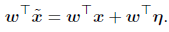
Thus the activation function grows by the second term in the above equation. It is possible to maximise this increase due to max norm by assigning 
This value does not grow with the dimensionality of the problem. But with the changes in the activation function due to perturbations of the each unit of n dimensions. Thus for higher dimensional problems, we can make many minute increases in the input units leading to huge variation in the output analogous to an "accidental stenagraphy".
This shows that given a linear model have a threshold dimensionality, it can generate adversarial examples. Most previous works and explanations were based on the hypothesized non linear behaviour of DNNs. Whereas our model is based on simpler linear structure of the model.
LINEAR PERTURBATION OF NON-LINEAR MODELS
Our view suggests that more linear the model, more faster is the generation of adversarial examples. However, we also hypothesized that the neural networks are too linear to resists adversarial geenrations. RELUs, LSTMs and maxout networks are intentionally designed to have linear behaviour to satisfy their funtion. Thus they are easy to optimize. But nonlinear models such as sigmoid functions are difficult to tune to exhibit linear characteristics. As we have already seen about the non linear nature of neural networks, this tuning further degrades the network.
The fast gradient sign mehod of generating adversarial images can be referred by the following equation.
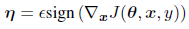
where theta is the parameters of a model, x is the input to the model, y the targets associated with x and J be the cost used to train the neural network. It should also be noted that the gradient can also be calculated using backpropogation in a better way. This method can easily fool many machne learning models.
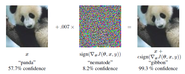
Consider the above example. An image initially clssified as panda is now being classified as gibbon and that too with very h
igh confidence. In case of MNIST test dataset, we were able to obtain error rate of 99.9% with a confidence of 79.3%. Also there exists many other methods to produce adversarial examples - rotating the image by a small angle ( also known as image augmentation). The generations of these adversarial examples by such cheap and simple algorithms prove our proposal of linearity.
ADVERSARIAL TRAINING OF LINEAR MODELS VERSUS WEIGHT DECAY
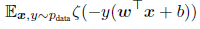
Here, we will be using fast gradient sign method to gain intuition about how these adversarial images are generated. If we train a model to recognize labels (-1, 1) with the function 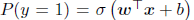 with logistic sigoid function, then the training involves performing gradient descent on the following function.
The above function is softplus function. Thus we can develop a function for generating the worst case perturbation by using the following function. This function is developed for simple logistic function.
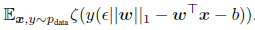
The function looks somewhat similar to L1 regularization with a very important difference that the L1 penalty is subtracted here instead of adding. This shows that the penalty values eventually disappers when the softplus function is able to generate images with high confidence. But this phenomenon is not true in case of underfitting as it will worsen the situation. Thus, the training during underfitting condition is worse than adversarial examples.
When we try to proceed multiclass softmax function, we find that L1 decay becomes still worse. Because it cannot find a single fast sign gradient which matches with all the classes of the data. Here, the L1 penalty become high which leads to high error on training as the model fails to generalize. In case of MNIST dataset, we got over 5% error. But this is for weight decay coefficient of 0.25. When we decrease the weight decay coefficient to very low, the training was successful but does not give any benefit of regularization.
ADVERSARIAL TRAINING OF DEEP NETWORKS
Universal approximate theorem states that any neural network with atleast one hidden layer will be able to mimic to represent any type of function either simple or complex. But with a given condition that the number of hidden units can be varied. Thus the common statement that the neural networks are vulnerable to adversarial examples is misleading. It is very clear to understand that though neural networks are able to represent any function why are they so vulnerable to adversarial training.
However, the universal approximate theoren does not say that the represented function will be able to wxhibit all the desired properties. Also, it never told that the generated function would be resistent to adversarial training.
Results from earlier studies have shown that the model training on a mixure of real and adversarial examples can achieve partial regularization. Regularization is a process to minimise the chances of overfitting. Training being performed on adversarial examples are different from that of data augmentation. Data augemtation includes processes such as translation to make sure that data that might be present in test set are also included in the training data.
We found that the fast gradient sign method with a modification of adversarial objective function was able to perform regularization better.

We used a constant learning rate of 0.5 throughout the experiments. Ths means that we continuously supply the adversarial examples to make them resist the current version of the model. Using this approach to train a maxout network with regularization and dropout was able to reduce error rate from 0.94% without adversarial training to 0.84% with adversarial training.
But we observed that the error rate doesnot reach 0. Thus, we made the two changes. First, we made the model larger using 1600 units per hidden layer from earlier 240 layers. But due to adversarial training, the model became slightly overfitted and gives 1.14% error in test set. As the progress was very slow, we used early stopping. The final training was done on 60000 examples. Five different runs are performed with different random seeds. One such trial had an error rate of 0.77%. The model also became slightly resistent to adversarial examples.
Earlier using fast gradient sign method, we got an error of 89.4% but with adversarial training the error rate fell to 17.9%. Adversarial examples are transferable given that they are robust enough. Adversarial examples generated via the original model yield an error rate of 19.6% on the adversarially trained model, while those generated via the new model yield an error rate of 40.9% on the original model. If an adversarial trained model misclassfies , it does with high confidence. Thus adversarial training can be viewed as a method to minimise the worst case erroe when the data is perturbed by an adversary. It can also be seen as a form of active learning where a heuristic labeller labels the data points to its nearby labels.
We could also make the network insensitive to changes that are smaller than the precision value. This is analogous to adding noise with the max norm during traning. However, noise wth zero mean and zero variance is very inefficient at preventing adversarial examples. Thus, the above calculated dot product will be zero which will have no effect but making the situation complex.
As the first order derivative of the sign function is zero or undefined throughtout the function, gradient descent on the adversarial objective function as a modification of the fast gradient sign method does not allow the model to anticipate how the adversary will react to changes in the parameters. If we instead use adversarial examples with small rotation or changed gradient, as the perturbation process is differentiable, it takes adversary into account.
We may ask sometimes whether it is better to perturb the input or hidden or both. As per the earlier results, it is better is to perturb the hidden layers. But as per our results, it is better to perturb the input layer. In our cases, perturbing the final hidden layer especially never yielded better results.
DIFFERENT KINDS OF MODEL CAPACITY
We, humans naturally find it difficult to visualize higher dimensions above three. We cannot determine or understand the functioning and changes happening at that situations. We also have a myth that low capacity models always have low confidence score while predicting. But it is not always true. But, for example, RBF networks are able to obtain higher confidence scores with a low capacity. Its mathematical expression is mentioned below.

WHY DO ADVERSARIAL EXAMPLES GENERALIZE?
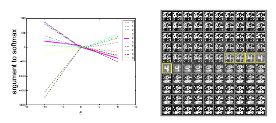
One important thing to note is that the example generated by one model also misclassifies other models. This stays true for different models even with different architectures and even disjoint training data. However, theory of non-linearity or overfitting cannot explain this behaviour as they are specific to a particular model or training data. But it can be well understood using the hypothesis that these adversarial examples for any data are tiled within the data itself just like the occurances of rational numbers within the real numbers. This happens because they are common but occur only at specific locations. THis statement is further backed by the following image. It explains the occurances of adversarial examples for various classes. It is easy to note that there exist a direction for each class. This explains the generality of the network.
In oredr to test this hypothesis, we generated adversarial examples on deep maxout networks and classified using shallow softmax network and shallow RBF network. While shallow softmax networks were able to classify maxout's class 84.6% of the time, shallow RBF was able to classify it 53.6% of the time. Our hypothesis cannot back these results but explain that a significant portion of the misclassifications are common to both of the models.
ALTERNATIVE HYPOTHESES
Due to the failure of our hypothesis, we now develop some alternate hypothesis. One such thing is to make the training process more constraint or make the model to understand the differences between real and fake images. In case of MP-BDM (Multi-Prediction Deep Boltzmann Machines) model, when working on MNIST data gave an error rate of 97.5%. This exolains that being constraint doesnot improve any chances.
Another hypothesis is that individual models have these strange behaviours but averaging over multiple models can lead to elimination of these adversarial examples. But while experimenting, these ensemble methods gave an error rate of 91.1% . When the perturbation is made to only one model of the ensemble methods, the error rate falls to 87.9%. This shows that ensembling provides only limited restraints to adversarial examples.
RUBBISH CLASS EXAMPLES
Another concept that is related to adversarial examples is the examples drawn from a “rubbish class.” These examples are degenerate inputs that a human would classify as not belonging to any of the categories in the training set. This gives its name. We should not include these in the training data as it might affect the number of false positives leading to inefficient model performance.
SUMMARY AND DISCUSSION
The observations of this paper are:
- Adversarial generation is due to linear property of high dimensional dot products.
- The generalization of adversarial examples is due to alignment of weight vectors of models with all other models.
- The direction of application of perturbation is an important factor in adversarial example generation.
- As the adversal depends mainly on direction, they also occur for clean examples when applied.
- We have developed methods to generate adversarial examples.
- We observed that this method performs better regularization than dropouts.
- Models that are easy to optimise are also easy to perturb.
- Linear models fails to resist this effect. Only models with atleast one hidden layers were able to resist this.
- RBF (Radial Basis Function) networks are resistant to adversarial examples.
- Ensembles are not resistant to adversarial examples.
Though most models with sigmoid, maxout, ReLU, LSTM etc. are highly optimised to saturate without overfitting, the property of linearity causes the models to ultimately have some flaws. Though most of the models correctly labels the data, there still exists some flaws. Thus we should try to identify those specific points that are prone to these generation of adversarial examples.
References
- Paper (PDF) at ArXiv
- Deep Neural Networks are Easily Fooled: High Confidence Predictions for Unrecognizable Images by Murugesh Manthiramoorthi at OpenGenus
- One Pixel Attack for Fooling Deep Neural Networks by Murugesh Manthiramoorthi at OpenGenus
- Machine Learning topics at OpenGenus