
Get this book -> Problems on Array: For Interviews and Competitive Programming
This article is a simplified version of "One Pixel Attack for Fooling Deep Neural Networks" by Jiawei Su et al. In this article, we will learn how a state of art Deep Neural Network can be fooled by varying only a single pixel in the images.
This paper (by Goodfellow) summarizes the ideas of Adversarial examplesIntroduction
Though the advancements in deep learning models are going fast and in a positive way, there still exists certain loopholes where even a high performance models can misclassify images.A small change in the images which are irrecognizable to humans can cause DNNs to place images under wrong class. These images which are generated by certain effective algorithms are called Adversarial Images.
In the earlier mentioned techniques, they have made huge or visible changes to the image to create adversarial images for fooling the DNNs. But, we are making only a small variation that is not perceptible to human eyes. This investigation helps us learn new insights about the geometric characteristics and overall characteristic of DNNs in high dimensional space.
Advantages
We are using Kaggle CIFAR-10 dataset on three different DNN architectures such as AllConv, NiN and VGG. Instead of making more changes, just changing a single pixel carries a lot of advantages. They are given below.
1. Effectiveness
Just by modifying a single pixel, we are able to obtain 68.71%, 71.66% and 63.53% respectively. Each natural images can be perturbed to generate 1.8, 2.1 and 1.5 other classes respectively for each architectures. While doing this experimentations with BVLC AlexNet model, we got 16.04% success rate.
2. Semi-Black Box Attacks
It requires information only about the probability label. It does not need any values of gradients, network structures etc. Our model is also very simpler compared to other existing models. It directly focuses on increasing the probability label value of the target classes.
3. Flexibility
It can attack many DNNs even if the network is non differentiable or even if the gradient is difficult to calculate.
4. Analyze the vicinity of natural images
It is also useful in analyzing the vicinity of the original image. In general prior other works, they have used universal perturbation which searches for modified pixel in the form of spheres from the natural images. But, we have used a very particular case where we focus on only one pixel. Theoretically, it helps us to have better understanding of the CNN input space.
5. A measure of perceptiveness
None of the earlier proposed methods can guarantee that the modifications made are imperceptible. But as we have replaced the perturbation vectors with a limited number of pixels, we can assure that the modifications made are very minimal.
Problem Description
Here, generating adversarial images can be seen as analogous to optimization problem with additional constraints. Let f be the target image with n-dimensional features x and is correctly classified to the original class. Then, the probability of the image belonging to the particular class is f(x). The vector e(x) is an additive adversarial perturbation of the natural image of the target class adv with the limitation of maximum modification of L. L is always measured by the maximum modification of e(x). The goal is to find the optimized solution for the following equation.
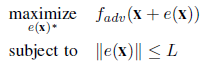
The objective is to find two values.
- Which dimension of the natural image is to be perturbed
- The corresponding strength of modification for each dimension
For our approach, the equation can be modified as shown below.
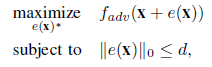
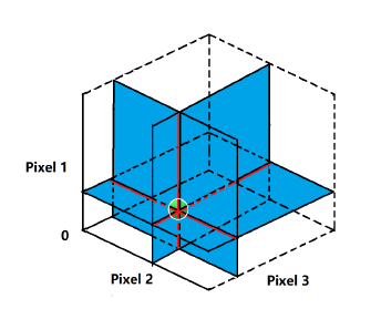
where d is a very small number. In the case of one pixel attack, the value of d is 1. One pixel attack can be defined as the process of modifying one dimension parallel to the axis of one of the n dimensions. Similarly, a 3 (5)-pixel modification moves the data points within 3 (5)-dimensional cubes. Actually speaking, one pixel attack makes modifications to the image in the required direction. It is clearly observed through the below image.
Differential Evolution
As mentioned above this is an optimization problem. Complex optimization problems can be solved by a population based optimization algorithm called differential evolution. It belongs to the general class of Evolutional Algorithms. It has the ability to keep the diversity during the selection phase which is a great advantage when compared to other generic Evolutional Algorithms or other gradient based solutions. Thus here, both the parent and the child images are compared to make sure that the diversity is maintained. At the same time, fitness values of the images can also be improved. Also, here the optimization does not use the gradient information. Thus, this method can be used for situations that are not differentiable. The usage of Differential Algorithms has the following advantages.
1. Higher probability of Finding Global Optima
Unlike Gradient Descent or Greedy Algorithm, the chances of falling prey to local minima instead of finding the global minima is relatively less. Since this process is strictly restricted to only one pixel modification, it is highly hard for such mishaps to occur.
2. Require Less Information from Target System
This optimization algorithm does not require information about differentiation unlike other algorithms like quasi Newton method and Gradient Descent. Thus this can be used even if the networks are non differentiable or even if the gradient is too difficult to process.
3. Simplicity
The algorithm does not require information about the model used for classification. All it requires is the probability of the label.
Methods and Strings
We encode the perturbations made into an array which is optimized by using Differential Evolution. One array of solution consists of a fixed number of perturbations and each perturbation is a tuple holding five elements - x, y coordinates of the pixel and the RGB value of the particular pixel. Each perturbation modifies one pixel. Initially, there are 400 arrays and after each iteration another 400 arrays are formed. This process follows the following Differential Evolution formula.
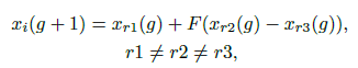
where xi is an element of a particular perturbation, r1, r2 and r3 are random numbers, F is the scale parameter set to 0.5, g is the current iteration at that time. After each generation, each element fights with the parent element based on the index and the winner proceeds to the next iteration. The maximum iteration is set to 100 and the early stop is turned on if the probability reaches 90%.
Evaluation
The evaluation process is performed on CIFAR and ImageNet datasets. The metrics used to measure the effectiveness of the attack are explained below.
1. Success Rate
In case of non-targeted attacks, it is defined as the percentage of adversarial images that are wrongly classified. In case of targeted attacks, it is defined as the probability of perturbing a natural image as a particular class.
2. Adversarial Probability Labels
The sum of the probability of the labels after each successful perturbations divided by total number of successful perturbations. The value shows the confidence of the target class when misclassifying it.
3. Number of Target Class
It counts the total number of natural images that can be successfully perturbed to a certain number of target classes. By knowing the unsuccessful perturbation, the effectiveness of the non-perturbed class can be determined.
4. Number of Original-Target class pairs
It counts the total number of times each original-destination class pair has been attacked.
Kaggle CIFAR - 10 dataset
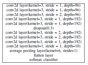
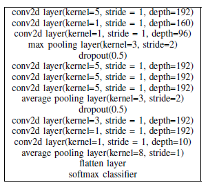
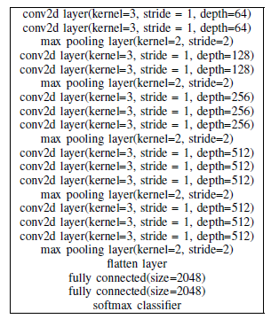
We train the dataset using three different networks - All Convolution Network, Network in Network and VGG16 Network. whose structures are shown below respectively.
Both targeted and non-targeted attacks were performed on all the three networks. Thus, for each of the six attacks, 500 random images were chosen from the CIFAR 10 test dataset.
In addition to these experiments, we also conducted an All Convolution Network on 500 adversarial images using three and five pixel attacks. Even if the perturbed image shows a false result other than the original class, then it is a success for the process. Thus, we were able to generate 36000 adversarial images.
ImageNet dataset
In case of ImageNet dataset, we perform only non targeted attacks on all the above mentioned networks. In order to execute this, we use a fitness function whose purpose is to decrease the probability value of an image for its true class. The experiment is performed on BVLC AlexNet using 105 images from ILSVRC 2012 test set selected randomly with same number of evaluations throughtout the process. The images are resized to 227 x 227 before inputting.
Results
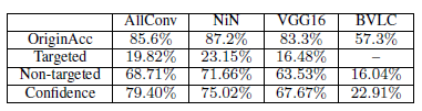
After the completion of the experiments, the success rate and the adversarial probability values for one pixel attack on all the three networks on CIFAR 10 dataset and BVLC are shown below.
The heatmaps for the original - target class pairs are shown below.
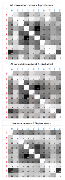
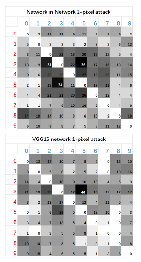
Here, the numbers 0 to 9 indicates their respective classes: airplane, automobile, bird, cat, deer, dog, frog, horse, ship, truck. Now, let us look at the evaluation parameters for the experiments performed.
1. Success rates and Adversarial Probability labels
The success rates on different networks show the generalized effectiveness of the perturbation on CIFAR 10. Basically, each natural image can be perturbed to about to different target classes and it can be increased to about three based on the network. Confidence values obtained by dividing adversarial probability values by the success rate for one, three and five pixel attacks respectively are 79.39%, 79.17% and 77.09%.
By viewing the results of ImageNet, we observe that the one pixel method is mostly able to fool large sized images. This shows that it generalizes well for large sized images. We were able to obtain 22.91% confidence. This is relatively low confidence. We have obtained this due to the fact that we have used a fitness function whose primary roles is to decrease the probability value of the target class. Other functions might yield different results.
2. Number of Target Classes
Look at the image below. It shows the attacks on different architectures.
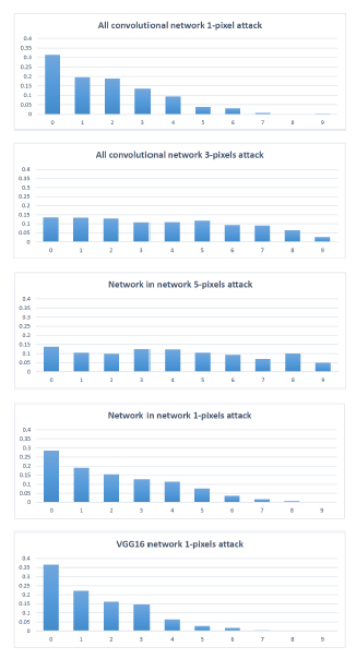
By observation, we find that with just one pixel attack, we were able to perturb the natural image to two or three classes. By increasing the number of pixel attacks, we were able to increase to the target classes. The above image proves that all the three networks are vulnerable to our approach. Thus, this proves that one dimensional perturbation is more than enough to generate adversarial images. With five pixel perturbation, we are even able to fool eight target classes.
3. Original-Target Class Pairs
Some specific original-target class pairs are easily vulnerable compared to others. For example, the images of cats are easily perturbed compared to dogs and automobiles. This indicates that the data points are specific to each classes. Specifically speaking about one pixel attack, certain target classes are more hard as their data points are difficult to obtain. Data points of a specific class does not coincide with other classes. Also, while observing the above heatmaps, we can see their symmetric nature. This shows that each class has similar number of adversarial images derived from each other classes.
4. Time complexity and average distortion
Number of evaluations is used to measure the time complexity. Here, the number of evaluations is calculated by the product of number of entries in the input array and the number of generations. We also calculate the average distortion of each pixel attacked by observing the difference on the RGB values of each pixel before and after attack. The results are shown below.
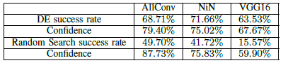
5. Comparing with Random One-Pixel Attack
Now, we are comparing our proposed method with random attack to make sure that if Differential Evolution actually helps in one pixel non targeted perturbation. The comparison is done on Kaggle CIFAR 10 dataset and the results are shown below.
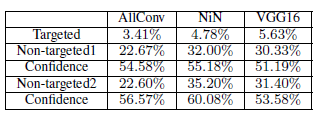
Opposing the Differential Evolution, a random search method repeats 100 times, each time randomly modifying each pixel of the image thereby changing it's RGB value. The highest probability of all the 100 iterations are chosen as the confidence of the attack. With same number of evaluations for both the Differential Evolution and random search, Differential Evolution is found to be more efficient especially in case of VGG6 network.
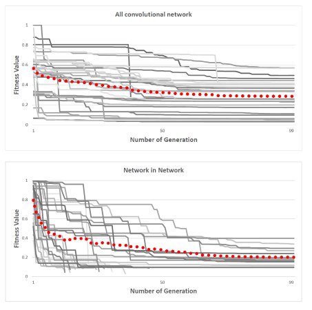
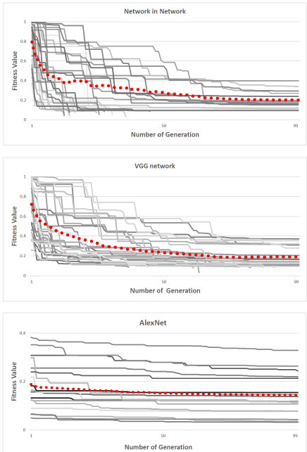
6. Change in Fitness Value
Now, we perform experiments to observe the change in the fitness values over different networks. In the images given below, the 30 (or 15) curves comes from 30 (or 15) randomly chosen CIFAR 10 test images. The fitness value of each image is the probability value of the true class for each image. The fitness values decreases after each generation. Sometimes, the value decreases abruptly while sometimes it decreases slowly. It is also evident that BVLC network is slightly harder to fool because of small decrease in fitness value with generations.
Conclusion
Adversarial Perturbation
Here, the frequency of changes in the image labels are observed for every generations. We also showed that it is possible to move the data points to find the position where the value changes. The results also suggest that small additive changes to multiple dimensions of the image finally leads to huge changes. It is found from the experiments that the CNN perturbed by one pixel attack are more generalized to images of all sizes and all types of networks. It uses lower number of DE iterations with huge initial array. Implementation of more advanced algorithms such as Co-variance Matrix Adaptation Evolution Strategy may also yield same results.
Robustness of One-pixel Attack
Some recent improvements is able to detect adversarial perturbations at all levels. However, all those methods add another layer to the network which slows it down. Detecting adversarial images have huge legal and emotional advantages. But still, neural networks are not able to identify similar images with small perturbations. WE should discover or develop novel methods to improvise the situation.
Resources
- Read the original paper here (PDF) on ArXiv