Open-Source Internship opportunity by OpenGenus for programmers. Apply now.
In this article, we will explore into sample problems and formulate it as a linear programming problem. We have considered three problems:
- Product Mix Problem
- Transportation Problem
- Flow Capacity Problem
Before we look into linear programming, let us have a quick look at Mathematical progamming, which is a superset of linear programming.
Mathematical Programming
Mathematical Programming is used to find the best solution to a problem that requires a set of decisions about how to best use a set of limited resources to achieve a state goal or objective.
The different steps involved in mathematical programming is as follows:
- Convert the problem into a mathematical model.
- Explore different solutions of the problem.
- Find the most optimal solution.
Linear programming model
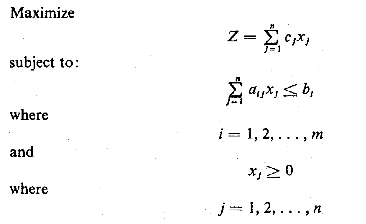
Linear programming requires that all the mathematical functions in the model be linear functions.
If the different decision variables are X1, X2, X3, .... Xn
Objective function or linear function is Z

Developing a Linear Programming Model
Steps
- Determine the objective function Z and the constraints in terms of the decision variables.
- Solve the problem by finding out a suitable combination of decision variable values that optimize the criterion function while satisfying all the constraints imposed on the problem. Here, one can use different methods of solving: Simplex method.
Examples of Linear Programming Model
The problems that can be solved using the linear programming model can be broadly classified into the following types:
Product Mix Problem
Here, a manufacturer has fixed amount of different resources that can be combined, in different combinations, to produce different products. The problem here is to find that combination of the products produced that would maximize the total income, given the constraints.
Example Problem Statement
XYZ Company produces two products: I and II. The raw material requirements, space needed for storage, production rates, and selling prices for these products are as follows, along with their constraints
| Requirements | Product 1 | Product 2 | Constraints |
|---|---|---|---|
| Storage space ft2/unit | 4 | 5 | <= 1500 |
| Raw material lb/unit | 5 | 3 | <= 1575 |
| Production rate units/h | 60 | 30 | <= 7 hours |
| Selling price | 13 | 11 | Maximize! |
Here, the company wants to determine how many units of each product to produce per day to maximize its total income.
Solution
Let x1 and x2 be the number of units of products I and II, respectively, produced per day.
Therefore the linear programming problem can be formulated as follows:
Maximize Z = 13 x1 + 11 x2
subject to the constraints:
- Storage space: 4 x1 + 5 x2 ≤ 1500
- Raw material: 5 x1 + 3 x2 ≤ 1575
- Production rate: x1 / 60 + x2 / 30 ≤ 7 or x1 + 2 x2 ≤ 420
- Non negative constraints: x1, x1 >=0
Transportation Problem
In this problem, a product is to be shipped from shipping origins and received at each of n shipping destinations. The cost of shipping a unit from each origin-destination pair is known for all combinations of origins and destinations. Here, the problem is to determine the amount to be shipped from each origin to each destination, in order to minimize the total cost of transportation.
Example Problem Statement
There are two warehouses A and B of capacities 100 quintals and 50 quintals respectively. They transport to three ration shops D, E and F whose requirements are 60 quintals, 50 quintals, and 40 quintals respectively. The transportation cost per quintal (in rupees) is as follows:
| From/To | A | B |
|---|---|---|
| D | 6 | 4 |
| E | 3 | 2 |
| F | 2.5 | 3 |
Here, we need to reduce the cost required for transporting the goods between the warehouses and the ration shops, and determine the number of quintals transported between each pair of warehouses and ration shops.
Solution
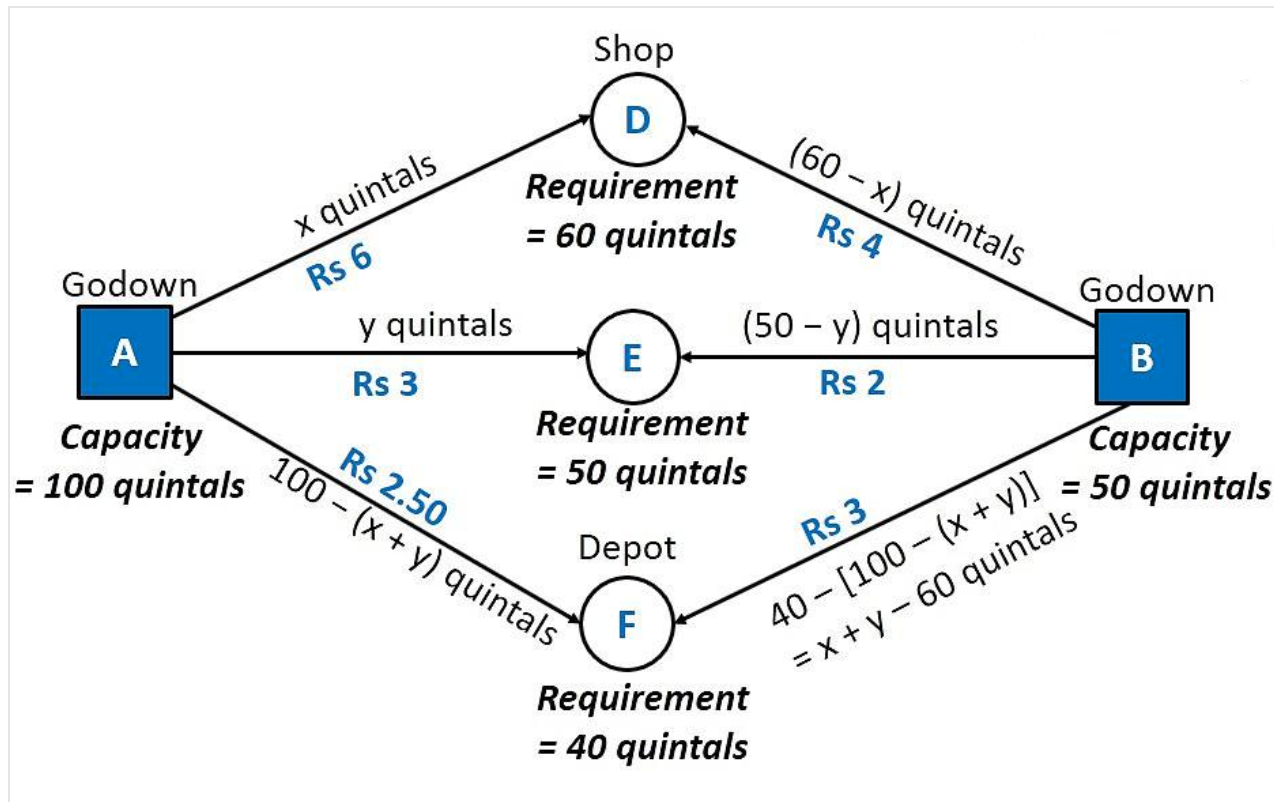
First we construct the diagram as follows:

Let
- x1 be the number of quintals transported from A to D
- x2 be the number of quintals transported from A to E
Taking into account the requirements of each ration shop, and the capacity of the godowns, Number of quintals transported between each pair of warehouses and ration shop is as follows:
| From/To | A | B | Requirement |
|---|---|---|---|
| D | x1 | 60 - x1 | 60 |
| E | x2 | 50 - x2 | 50 |
| F | 100 - x1 - x2 | 50 - (60 - x1) - (50 - x2) = 40 - (100 - x1 - x2) = x1 + x2 - 60 | 40 |
| Capacity | 100 | 50 | Minimize! |
Therefore, since all the quantities transported have to be 0 or positive, the constraints are as follows:
- x1 , x2 >= 0
- 60 - x1 >= 0
- 50 - x2 >= 0
- 100 - x1 - x2 >= 0
- x1 + x2 - 60 >= 0
The objective function denotes the cost of transportation
Z = 6 * x1 + 4 * (60 - x1) + 3 * x2 + 2 * (50 - x2) + 2.5 * (100 - x1 - x2) + 3 * (x1 + x2 - 60)
Z = 2.5 x1 + 1.5 x2 + 410
Therefore the linear programming problem can be formulated as follows:
Minimize Z = 2.5 x1 + 1.5 x2 + 410
subject to the constraints:
- x1 + x2 >= 60
- x1 + x2 <= 100
- x1 <= 60
- x2 <= 50
- x1 , x2 >= 0
Flow Capacity Problem
This problem deals with the flow of commodities like traffic, water, information, cash, etc. from one point to another through a network with branches having flow capacities. The problem is to determine the maximum flow, or capacity of the network.
Here, we would be given a set of nodes with branches connecting them. Each branch has a flow capacity (that is the maximum flow allowed through that branch). We would also be given a source node and a sink node. The objective here is to maximize the flow between the source and the sink.
The variables are the flow through each branch of the network. The constraint is that the flow through each branch should be positive and less that or equal to the maximum flow allowed through that branch. Also at every node, the total flow flowing into it is equal to the total flow flowing out of it. The objective function is the sum of all flows flowing out of the source node (to nodes that can reach the final sink node).
With this article at OpenGenus, you must have the complete idea of formulating a linear programming problem. Enjoy.
