Reading time: 30 minutes | Coding time: 10 minutes

Gradient Boosting is a machine learning algorithms used to predict variable (dependent variable). It can be used both in regression and classification problem. Like other machine learning algorithms gradient boosting has its own intution.

Gradient Boosting algoriths are determined as optimization algorithms as they try to execute the task with least cost. It produces a prediction model in the form of an ensemble of weak prediction models, typically decision trees. It working is also somewhat related to gradient descent. It follows a loss function to minimize the error. So it aims to generate least residual as possible. It aims to covert a weak learner to strong learner. As many of machine learning algorithms have not capability to predict a certain variable. Hence they are considered weak learners. So for cases like this gradient boosting came into play.

It generally assigns weights to each record in dataset and also considering predcition with most frequent values of that record. It generally follows the ensemble learning rules like random forest. So it uses number of decision trees for its implementation and to predict the variable.

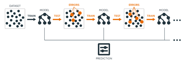
Gradient Boosting generally consist of various weak classifiers to form a strong classifier. For that purpose we use decision tree as they have small depth which led to high bias in each of them.

Types of Boosting Algorithms

There are two types of Gradient Boosting algorithms namely:

1. XGBoost
2. AdaBoost

1. XGBOOST

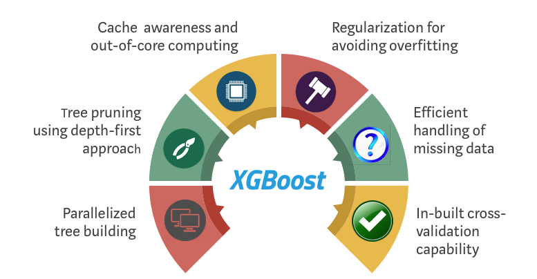
It is an implementation of gradient boosting to provide better speed and performance. It is decision tree based ensemble machine learning algorithm.

Working of XGBOOST:

Lets suppose we have an dataset with dependent variable and each record has an output feature which can be considered as dependent variable.
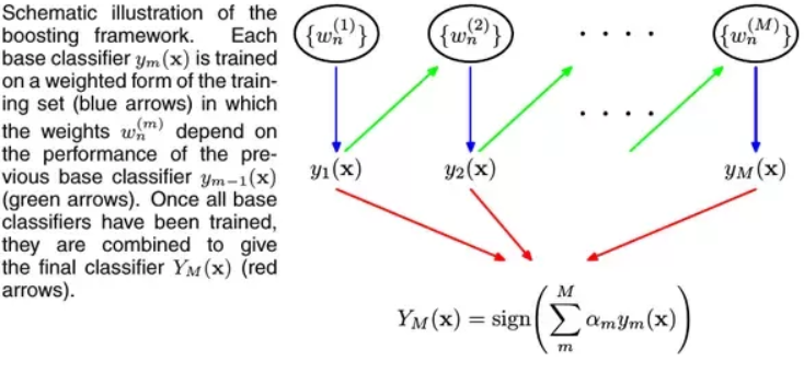
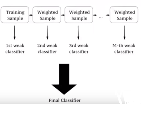
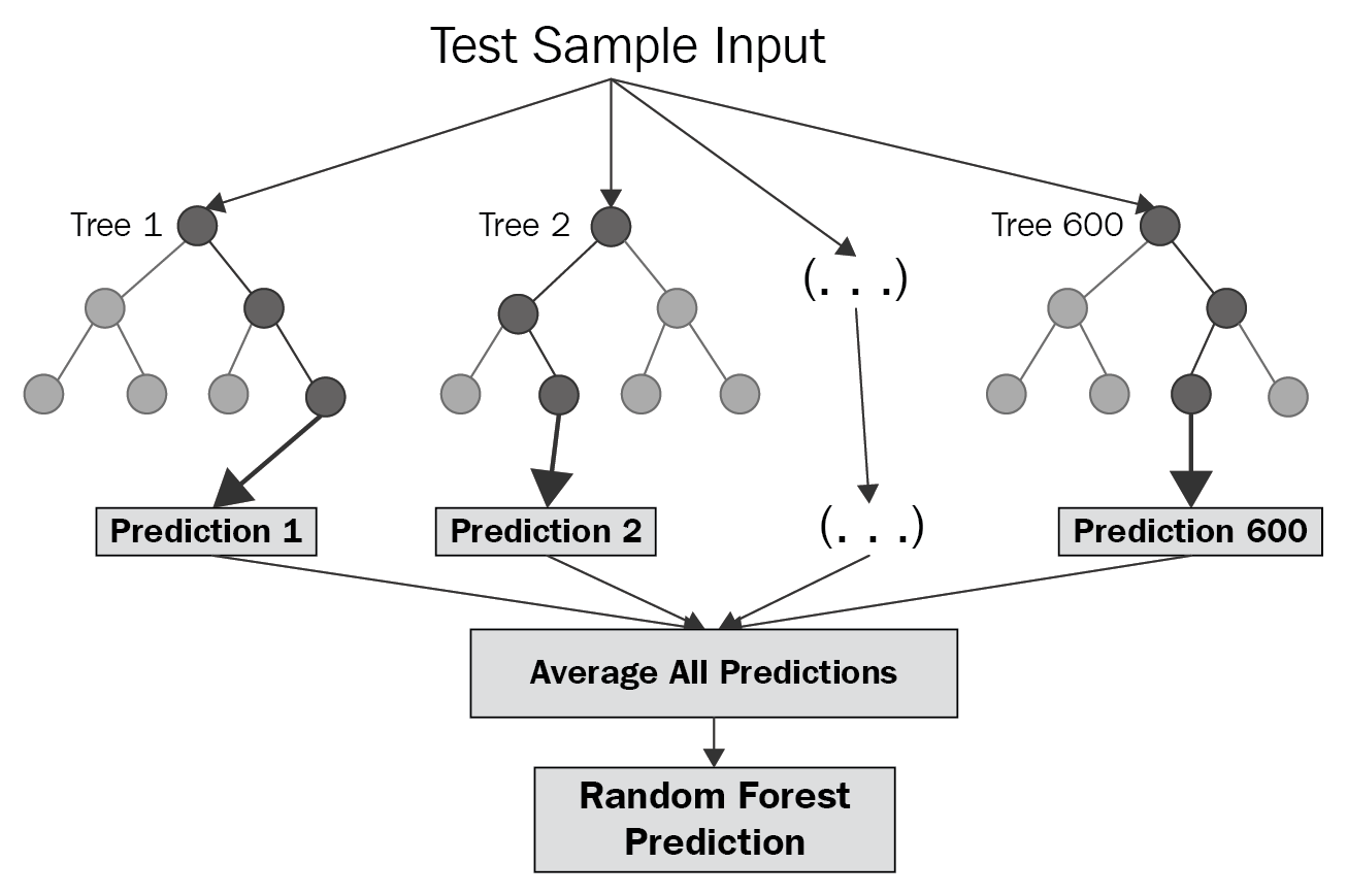
Now in case of random forest decision tree are implemented parallel way, we train our model and achieve accuracies from each model. But in XGBoost we generally we have decision tree sequentially. Hence this is called sequential ensemble technique.

Random Forest:

XGBoost:

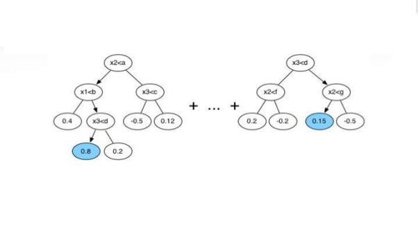
Now we will assign some weights to each record and these weights are similar to each other. These weights signifies that what is probability to selected be decison tree for training process. Each decision tree will have its own sets of records after determining their probability. After that decision tree will predict the dependent variable.

Now after predicting the variable, it will check with actual record that whether predicition is correct or not. If the prediction is wrong for a variable the weight assigned to that record will get updated. Hence this is called as weak classifier model. And after updation they are feeded to decison tree model and predictions are generated again. If there are again wrong prediction weights are updated again for that record. And all this defining of model and generating prediction happends sequentially.

Now at last we will have various classifiers and each will be called weak classifier. In case of predicting data from test data, each classifier will predict its own values like classifier 1 predicts 0, classifier 2 predicts 1 and classifier 3 predicts 1. Then most predciting value be considered for that record. In this case it is 1. And in case of continious values, the mean value of all will be considered.

Since XGBoost uses decision tree upto some depth than there will be High Bias and Low Variance.

Implementation

For the purpose we will implement XGBoost on a random dataset.
The dataset contains bank details of customers

After performing necessar data cleaning and processing we recieved final dataset. Now we implement our XGBoost model

X=train_df.drop('Survived',axis=1)
Y=train_df['Survived']

from sklearn.model_selection import train_test_split
x_train,x_test,y_train,y_test=train_test_split(X,Y)

from xgboost import XGBClassifier
model = XGBClassifier()
model.fit(X_train, y_train)

y_pred=model.predict(x_test)

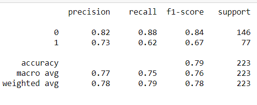
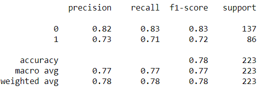
Evaluation:

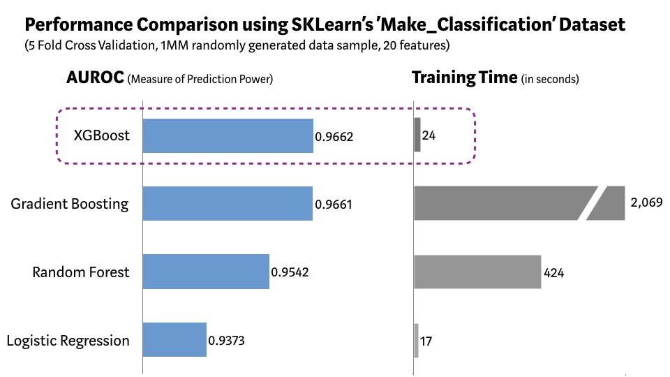
XGBoost predicts with greater accuracy and with less time complexity as compared to other machine learning algortihms

2 AdaBoost

It is an another boosting algorithm which is also called adaptive boosting. It follows the same principle of boosting algorithms like to convert a weak classifier to strong one.

Mathematical representation:

f_m stands for the m_th weak classifier and theta_m is the corresponding weight

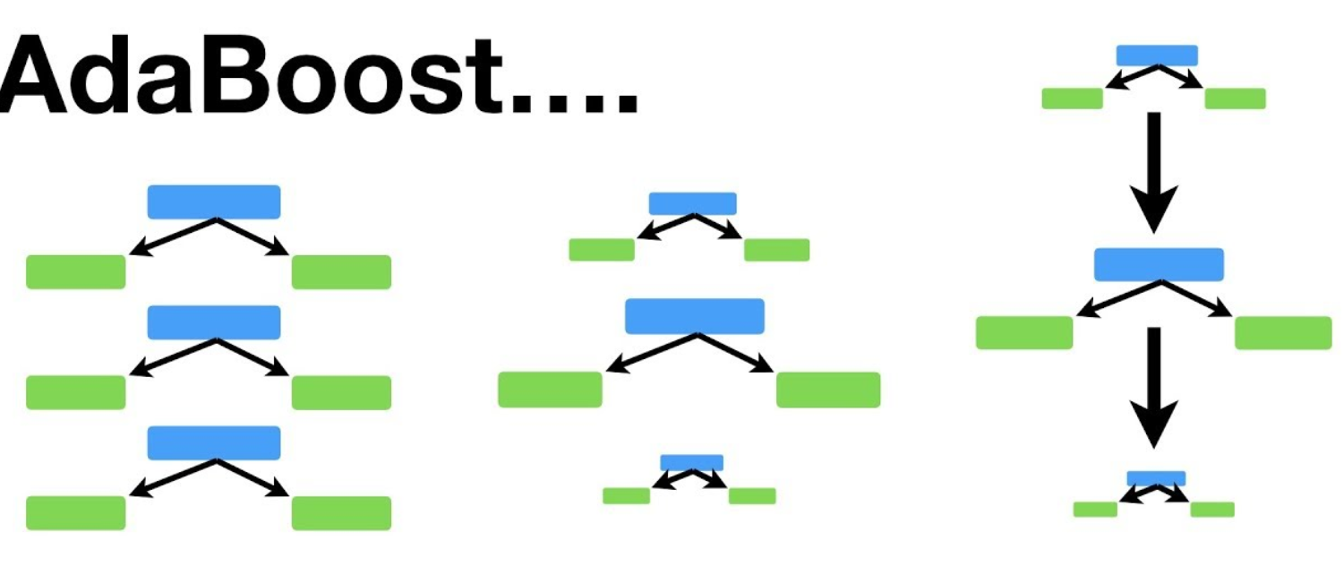
In random forest, there are various trees of different depths but in AdaBoost there are trees with one root and 2 node leaf. Their depths are fixed for all trees. This is called stump. Hence it is considered forest of stumps. But this means they can only consider one feature in their stump and hence they are called weak learners. This is where work of AdaBoost begins. In random forest, each tree has equal value for their vote but in forest of stumps made of AdaBoost some stumps has more value in their votes than other. The order of stumps also matters as error made by stump cannot be made by second as they learn from their previous ones.

3 Rules followed by AdaBoost:

• AdaBoost combines lot of weak learners to make classification. The weak learners are always almost stumps.
• Some stumps get more say in classification than others
• Each stump is made by taking previous stump mistake taken in account

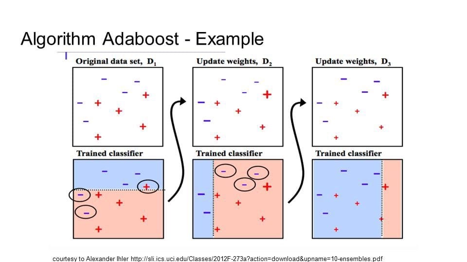
Like XGBoost, a sample weight is assigned to each record with similar value at starting. These weights will change to guide how next stump will be created. The first will be created on feature which is least correlated to dependent variable than others. This is done by calculating the ginni index by considering each feature in stump. Feauture with lest ginni index will be the first stump. Now we have to determine how much this feature will matter in final classification. After that we will determine the total error of each stump and amount of error will determine their say in final classification.This can be determined as:

So we will modify the weights so the next stump will take the errors that current stump made into account. We will increse the weights of correctly classified samples and decreased for incorrect ones. We will determine new weights using this formula:

In case of incorrect negative of amount of say is considered. Since the sum of weights should always be the 1. Hence we normalize the new weights. Now we will use the new sample weights to form our next stump. This will be determined by calculating the ginni index of each feature. Now same steps willbe repeated as before for determing new weights. And this whole process will be repeated untill a stump of each feature is created.

Now the predcitions will determined by comparing the amount of say of stumps. We will add up amount of say of all those stumps which are considering one category and for others too. And will compare at last. Group of stumps with highest amount of say will be considered as prediction value.

Implementation

Now for implementing the code we will conseder the same dataset as before.
We will perform same cleaning and pre-processing steps.
To implement AdaBoost:

from sklearn.ensemble import AdaBoostClassifier
adaboost = AdaBoostClassifier()
adaboost.fit(x_train,y_train)

y_pred = adaboost.predict(x_test)

Evaluation:

With this, you will have the complete knowledge of Gradient Boosting in Machine Learning. Enjoy.