
Get this book -> Problems on Array: For Interviews and Competitive Programming
Reading time: 35 minutes | Coding time: 10 minutes
In this article, we have explored how we can classify text into different categories using Naive Bayes classifier. We have used the News20 dataset and developed the demo in Python.
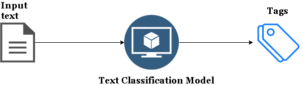
Text Classification
As the name suggests, classifying texts can be referred as text classification. Usually, we classify them for ease of access and understanding. We don't need human labour to make them sit all day reading texts and labelling categories. We have Machines !!
How can we classify?
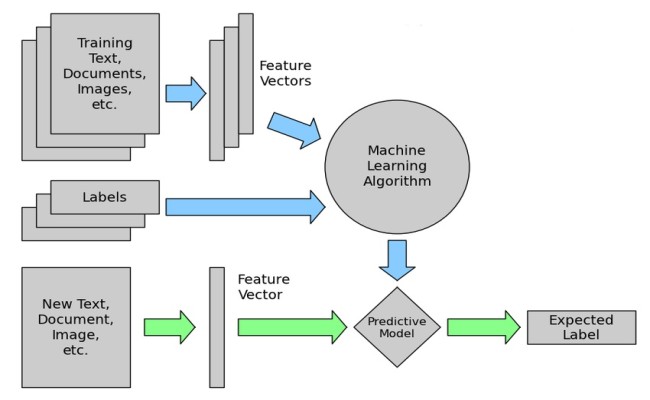
The trick here is Machine Learning which requires us to make classifications based on past observations (the learning part). We give the machine a set of data having texts with labels tagged to it and then we let the model to learn on all these data which will later give us some useful insight on the categories of text input we feed.
The general workflow for this task can be described as,
Naive Bayes
We are going to use Naive Bayes algorithm to classify our text data.
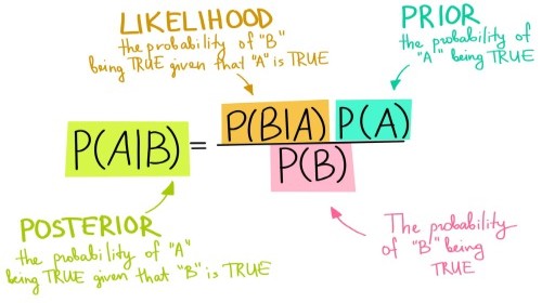
It works on the famous Bayes theorem which helps us to find the conditional probabilities of occurrence of two events based on the probabilities of occurrence of each individual event.
Consider we have data of student's effort level(Poor, Average and Good) and
their results(Pass and Fail).
| Effort | Result |
|---|---|
| Poor | Fail |
| Average | Pass |
| Average | Pass |
| Good | Pass |
| Good | Pass |
| Poor | Fail |
| Poor | Fail |
| Poor | Pass |
| Poor | Fail |
| Average | Pass |
| Average | Fail |
| Good | Pass |
| Average | Fail |
Student will fail if his efforts are poor. We want to check if this statement is correct. Then we can use Bayes Theorem as,
P(Fail | Poor) = P(Poor | Fail) * P(Fail) / P(Poor)
P(Fail | Poor) is read as Probability of getting failed given that the effort was poor.
P(Poor | Fail) = Number of students who failed with poor efforts / Number of students failed
= 4 / 6 = 0.66
P(Fail) = Number of students failed / Total students = 6 / 13
P(Poor) = Number of students with poor efforts / Total students = 5 / 13
P(Fail | Poor) = 0.66 * (6/13) / (5/13) = 0.66 * 6 / 5 = 0.792
This is a higher probability. We use a similar method in Naive Bayes to give the probability of different class and then label it with the class having maximum probability.
Let's take an example, where we want to tell if a fruit is tomato or not. We can tell it's a tomato from it's shape, color and diameter(size). Tomato is red, it's round and has about 9-10 cm diameter. These 3 features contribute independently of each other to the probability for the fruit to be tomato. That's why these features are treated as 'Naive'.
Classifying these Naive features using Bayes theorem is known as Naive Bayes.
Counting how many times each attribute co-occurs with each class is the main learning idea for Naive Bayes classifier.
How to use Naive Bayes for Text?
In our case, we can't feed in text directly to our classifier. Texts are huge, they have lots of words and various combinations so we use occurences of words in a single text data(i.e. term frequency-tf) and how many times that word comes across all text data (i.e. inverse document frequency-idf) and then we can generate feature vectors.
Feature vectors representing text contains the probabilities of appearance of the words of the text within the texts of a given category so that the algorithm can compute the likelihood of that text’s belonging to the category.
Once we are done finding likelihoods of various categories we find the category having maximum likelihood and there we have categorized our text!
For example, let's say you have a data set as :
| Document id | Content | Class |
|---|---|---|
| 1 | Nvidia GPU is the best in the world. | computer graphics |
| 2 | Nvidia is giving tough competition to AMD. | computer graphics |
| 3 | We were running our application with GTX 1050(High end GPU) still it didn't work then we realized the problem was with the OS. | computer graphics |
| 4 | GPU, Ganpat Pandey University, is located in Maharashtra. | not computer graphics |
| 5 | Please buy GPU from our store. | ? |
We can predict the class of last data by using Naive Bayes by considering the probability of important words,
Important words for com.graphics from the data can be considered as,
{Nvidia, GPU, AMD, GTX 1050}
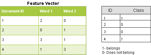
All words will have feature vectors of theirs representing their number of occurences in each record,
Nvidia -> [1; 1; 0; 0]
and so on.
P(computer graphics | GPU) = P(GPU | computer graphics) * (P(computer graphics) / P(GPU))
P(computer graphics) =
Number of records having class as computer graphics / Number of total records = 3/4 = 0.75
P(GPU) = Number of records having GPU / Total number of reccords = 3/4 = 0.75
P(GPU | computer graphics) =
Number of records having computer graphics with GPU in it / Total number of computer graphics' records
= 2 /3 = 0.66
P(computer graphics | GPU) = 0.66 * (0.75/0.75) = 0.66
This is greater than 0.5 so we can predict that this text data will be belonging to computer graphics.
Here, we have considered only one word GPU that is important in our test data but in real data we'll consider feature vectors of all words and then compute the probability for the class based on the occurences of all the non primitive words.
The main advantage is that you can get really good results when data available is not much and computational resources are scarce.
Making it work
For this task, we'll need:
- Python: To run our script
- Pip: Necessary to install Python packages
Once you are done with this, let's install some packages using pip, open your terminal and type in this.
pip install numpy
pip install sklearn
Numpy: Useful mathematical functions
Sklearn: Machine learning tools for python
Now, we are ready to get our hands dirty on the script
First, we'll begin by importing the libraries necessary.
import numpy as np
from sklearn.datasets import fetch_20newsgroups
from sklearn.feature_extraction.text import CountVectorizer
from sklearn.feature_extraction.text import TfidfTransformer
from sklearn.naive_bayes import MultinomialNB
from sklearn.pipeline import Pipeline
Here, we are importing the famous 20 News groups dataset from the datasets available in sklearn.
from sklearn.datasets import fetch_20newsgroups
Now, we define the categories we want to classify our text into and define the training data set using sklearn.
# We defined the categories which we want to classify
categories = ['rec.motorcycles', 'sci.electronics',
              'comp.graphics', 'sci.med']

# sklearn provides us with subset data for training and testing
train_data = fetch_20newsgroups(subset='train',
                                categories=categories, shuffle=True, random_state=42)

print(train_data.target_names)

print("\n".join(train_data.data[0].split("\n")[:3]))
print(train_data.target_names[train_data.target[0]])

# Let's look at categories of our first ten training data
for t in train_data.target[:10]:
    print(train_data.target_names[t])
Output:
['comp.graphics', 'rec.motorcycles', 'sci.electronics', 'sci.med']
From: kreyling@lds.loral.com (Ed Kreyling 6966)
Subject: Sun-os and 8bit ASCII graphics
Organization: Loral Data Systems
comp.graphics
comp.graphics
comp.graphics
rec.motorcycles
comp.graphics
sci.med
sci.electronics
sci.electronics
comp.graphics
rec.motorcycles
sci.electronics
We defined our task into several stages in the beginning. Here we are pre-processing on text and generating feature vectors of token counts and then transform into tf-idf representation.
Consider a document containing 100 words wherein the word ‘car’ appears 7 times.
The term frequency (tf) for phone is then (7 / 100) = 0.07. Now, assume we have 1 million documents and the word car appears in one thousand of these. Then, the inverse document frequency (i.e., IDF) is calculated as log(10,00,000 / 100) = 4. Thus, the Tf-IDF weight is the product of these quantities: 0.07 * 4 = 0.28.
i.e. Apply Vectorizer=> Transformer.
# Builds a dictionary of features and transforms documents to feature vectors and convert our text documents to a
# matrix of token counts (CountVectorizer)
count_vect = CountVectorizer()
X_train_counts = count_vect.fit_transform(train_data.data)

# transform a count matrix to a normalized tf-idf representation (tf-idf transformer)
tfidf_transformer = TfidfTransformer()
X_train_tfidf = tfidf_transformer.fit_transform(X_train_counts)
We fit our Multinomial Naive Bayes classifier on train data to train it.
# training our classifier ; train_data.target will be having numbers assigned for each category in train data
clf = MultinomialNB().fit(X_train_tfidf, train_data.target)

# Input Data to predict their classes of the given categories
docs_new = ['I have a Harley Davidson and Yamaha.', 'I have a GTX 1050 GPU']
# building up feature vector of our input
X_new_counts = count_vect.transform(docs_new)
# We call transform instead of fit_transform because it's already been fit
X_new_tfidf = tfidf_transformer.transform(X_new_counts)
Predict the output of our input text by using the classifier we just trained.
# predicting the category of our input text: Will give out number for category
predicted = clf.predict(X_new_tfidf)

for doc, category in zip(docs_new, predicted):
    print('%r => %s' % (doc, train_data.target_names[category]))
'I have a Harley Davidson and Yamaha.' => rec.motorcycles
'I have a GTX 1050 GPU' => sci.med
We now finally evaluate our model by predicting the test data. Also, you'll see how to do all of the tasks of vectorizing, transforming and classifier into a single compund classifier using Pipeline.
# We can use Pipeline to add vectorizer -> transformer -> classifier all in a one compound classifier
text_clf = Pipeline([
    ('vect', CountVectorizer()),
    ('tfidf', TfidfTransformer()),
    ('clf', MultinomialNB()),
])
# Fitting our train data to the pipeline
text_clf.fit(train_data.data, train_data.target)

# Test data
test_data = fetch_20newsgroups(subset='test',
                               categories=categories, shuffle=True, random_state=42)
docs_test = test_data.data
# Predicting our test data
predicted = text_clf.predict(docs_test)
print('We got an accuracy of',np.mean(predicted == test_data.target)*100, '% over the test data.')
We got an accuracy of 91.49746192893402 % over the test data.
With this, you have the complete knowledge of using Naive Bayes classifier from Text Classification tasks. Enjoy.