Graph Convolution Network (GCN)

Graphs and convolutional neural networks:

Graphs in computer Science are a type of data structure consisting of vertices ( a.k.a. nodes) and edges (a.k.a connections). Graphs are useful as they are used in real world models such as molecular structures, social networks etc.

Graphs can be represented with a group of vertices and edges and can also be represented by an image depicting the connection between the nodes. For example let’s consider a chemical molecule in which there are several atoms, the atoms are defined as nodes and the bond between them is defined as edges.

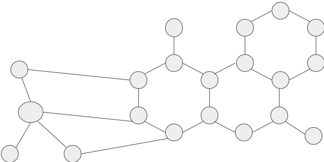
[Chemical Molecule]

The other types of graphs which are necessary to understand graph convolutional networks are:

1. Directed graph
2. Undirected graph

Directed graph:

A directed graph is a type of graph in which the nodes are connected to each other with the help of edges which have a direction associated with it. (A-> B -> C).

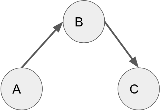
[A directed graph]
In the example above we see that the graph can be traversed from A to B and B to C but not from A to C.

Undirected graph:

An undirected graph is a type of graph in which the edges that connect the nodes, do not have a direction associated with it. They are not unidirectional and thereby the graph can be traversed in any direction. (A <-> B <-> C <-> A)

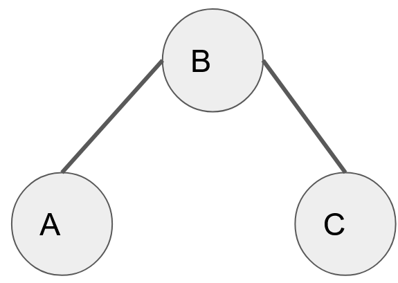
[undirected graph]
Another special type of graph which is also used to understand Graph convolutional networks is ‘complete graph’ - A complete graph is one in which all the nodes are connected to each other. Before we explore what is ‘Complete Graph’, lets understand more on how graphs help in Neural Network.

How do graphs help in a Neural Network:

The question now arises is how graphs would be fed into a neural network?
In order to understand how graphs are fed into a neural network we need to understand the following matrices:

1. Adjacency matrix (A):

An adjacency matrix is a type of matrix in which the elements would consist of either 1 or 0. It is a NxN matrix where ‘N’ denotes the number of nodes , it is also considered as a square matrix. Adjacency matrices are used to represent the edges which connect the nodes by representing it as a value of the matrices. In other words the elements of the matrix indicate if a certain pair of vertices are adjacent or not in the graph.

For example :

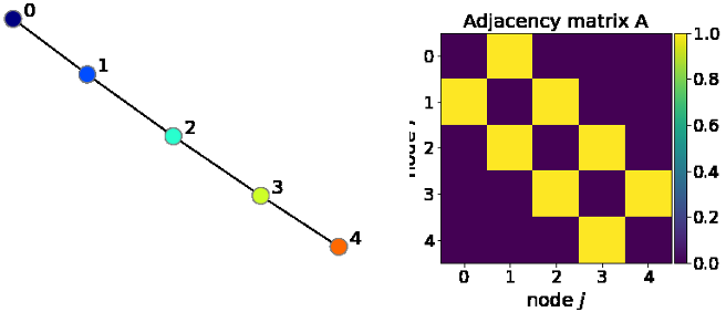
[Adjacency matrix]

In the above figure we see that the graph has 5 nodes , which then denotes that the matrix is of size [5x5]. Considering any matrix element Aij which has the value equal to “1” indicates that there is an edge between node ‘i’ and ‘j’. In the adjacency matrix above we see that there is a connection between node 3 and 4 (A34) which is yellow to represent 1 as they are connected. While node 0 and node 2 are not connected ,they are in purple representing 0. The above graph is an example of an in-complete graph as all the elements are not connected to each other.

2. Node Attribute Matrix (X):

The node attribute matrix is used to represent the features of each node. Supposing there are ‘N’ nodes and each node consists of ‘F’ features then the shape of the matrix is NxF.

Taking a look into the ‘CORA’ dataset, we will have a collection of words from several documents. The node attributes will be formed with the help of bag of words which denote the importance of a word in the document.

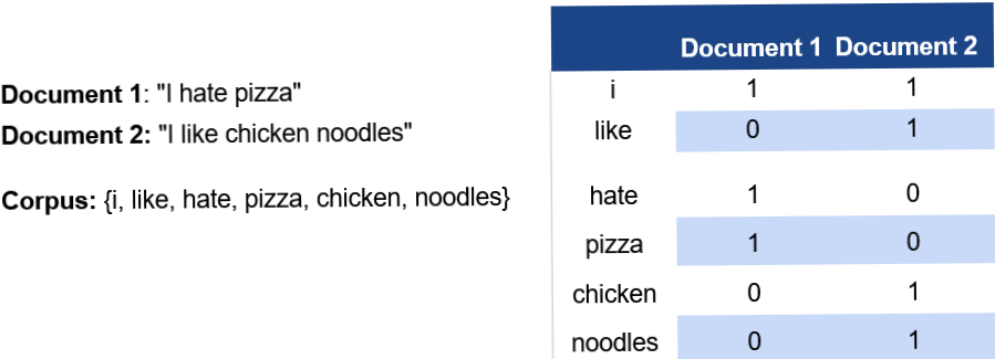
[Node attribute matrix]

3. Edge Attribute matrix:

Just like node attribute matrices in which the nodes had attributes similarly edges can have attributes as well, those matrices are called edge attribute matrices.

Now that we reviewed a brief summary of the basic graph theory, we will proceed to understand the graph neural networks.

Graph Neural Networks:

Taking an example of classifying the MNIST dataset , we would use CNN (convolutional neural network ) in which the images would be passed as input to the convolution layer and the kernel (filter) would scan over the image, taking into consideration the important features present in the image.

An image can also be represented as a graph in which:

1. A node will be represented as pixel
2. A feature of a node will be represented as a pixel value
3. An edge feature would be represented as a distance (euclidian) between each pixel present in the image.
   
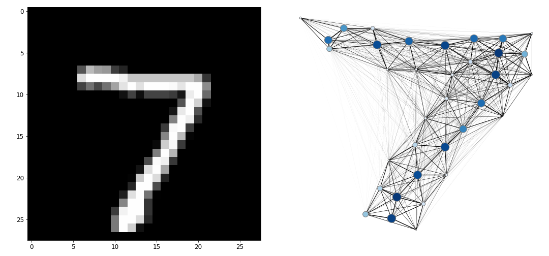
   [MNIST with graphs]

In CNNs the connection between each node is uniform and can be used to classify the image. CNNs tend to deal with data which has a ‘regular data structure’ i.e data which has euclidean distance such as 1D (text) and 2D (image), while GCNs tend to deal with data which has ‘non euclidean distance’ such as 3D images , chemical molecules etc. GCNs perform a very similar operation to CNNs in which the model learns the features by checking the neighbouring nodes.

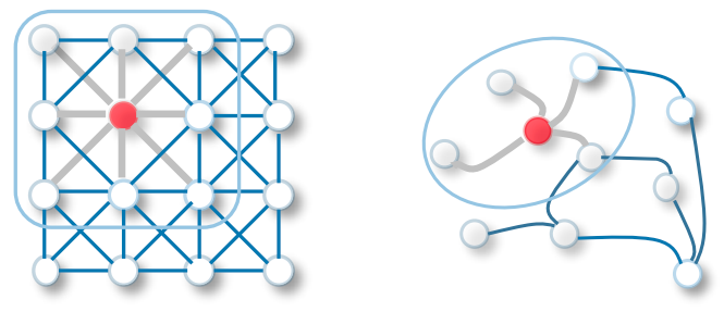
[2D convolution vs GCN classification]

GCNs can be broadly classified under two categorized based on the algorithms used:

1. The Spectral Graph Convolutional Networks
2. The Spatial Graph Convolutional Networks

The Spectral Graph Convolutional Networks:

Spectral graph convolution is based on signal preprocessing theory. In spectral graph convolutional networks we use eigen decomposition on the laplacian matrix of the graph.We can identify the clusters/sub-groups of the graph with the help of eigen decomposition which identifies the underlying structure of the graph. This entire process takes place in the fourier space.

A similar process has been seen in the dimensionality reduction technique called ‘PCA’ in which we understand the data with the help of eigen decomposition on the feature matrix.The difference between PCA and GCN’s is that smaller eigenvalues help in understanding the data better in GCN and it is the opposite in PCA.

In spectral graph convolutional networks , we take the adjacency matrix (say ‘A’) and use it in the forward propagation step in which it is added to the input features. ‘A’ is the matrix which is used to represent the edges present in the node in the forward propagation step. The addition of ‘A’ to the forward propagation step, allows the GCN to learn the features better as it reflects the connectivity of the nodes.The output can be seen as the result of the first GCN which is further propagated to the later layers with the help of the neighbouring nodes within the graph.

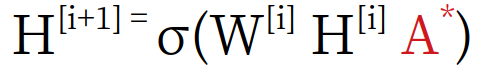
[Graph neural network formula]
The bias term is omitted for simplicity and A* is the normalized version which is used instead of A.
The laplacian matrix could be defined as L = I — D-½ A D-½
In the equation above we see that I → Identity matrix, D → diagonal matrix, A → adjacency matrix.

To sum up the entire process of spectral convolutions:

1. The first step is to transform the entire graph into a domain using eigen decomposition.
2. The second step revolves around the process of applying eigen decomposition to a specific kernel.
3. The third step is the process of multiplication between the spectral graph and the kernel.
4. The last step is to give the output in the original spatial region.

Below are some of the drawback of spectral convolution -

1. Dependency on the eigenvalues and the laplacian matrix, these two are required to perform the spectral convolution and due to this they become computationally expensive.
2. The time complexity for both the processes are O(n^2) for back propagation and O(n^3) for the calculation for eigen decomposition.
3. Spectral convolution needs the entire graph to be processed simultaneously which is not possible for large graphs such as social network graphs as they contain billions of nodes and edges.

The Spatial Graph Convolutional Networks:

Spatial convolution is pretty similar to regular convolution as in the way they spatially convolve over the nodes is nearly the same with regular convolution. Spatial convolutions create convolutions by clustering a node and its neighbors to form a new node. In other words they generate a new pixel from a pixel.

Spatial convolutions are considered to be the more moderate version of the graph convolutions. They work on the local neighbors of the node and help in understanding the properties of the node by using it’s ‘k’ local neighbors. The computational cost of spatial convolution is less compared to spectral convolutions.

The spatial convolution for a node can be expressed as a equation otherwise known as the ‘GCN propagation rule’ :

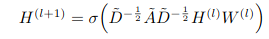
[Graph Propagation rule]
So this means that the h^(l+1) which are the hidden features at the next layer are defined as being a non-linear activation by the ~D , ~A , ~D term multiplied by the previous layer activation again multiplied with the weight matrix for this layer.

1. ~A is the adjacency matrix along with the self loops and this process is done so that each of the nodes in the graph include its own features in the next representation.This also helps with the numerical stability of the graph.
2. ~D is the degree matrix of ~A and is used to normalize nodes with large degrees.
3. D^½ and A^½ are used for symmetric normalization in which rather than doing the inverse degree matrix multiplied by the adjacency matrix, this takes the - ½ and apply it on each side of A

The terms ~D ^½ , ~A , ~D^½ is always of the size [n x n] because adjacency matrices are stored as [n x n] matrices where we have ‘n’ rows and ‘n’ columns and the entries to the matrix denoting the edges or sometimes edge weights. H’ is a matrix of dimension [n x γ] which is essential as the first term needs to match the dimension of the ~D , ~A , ~D term. The depth of the feature map can be controlled with the help of the second term ‘γ’, which could be used to shrink or expand the depth. W’ is a matrix of dimension [γ x γ] which helps in changing the output of the next layer.

After this we apply the activation function which could be Relu, sigmoid or tanh, the Relu function being mostly used.

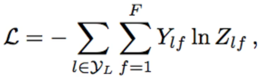
Computing Loss on Semi-Supervised Classification:

In semi supervised classification , how do we compute the loss?

[Loss on Semi-Supervised Classification]

During the processing of the features , it will eventually flatten it by ‘N’ in which N being the second dimension of the previous layer features, but an [N x 1] vector such that it flattens it out into a softmax probability distribution for each node. After this, the loss is taken on the labelled node because in semi supervised classification some nodes in the network will be labelled and others are not.

The key idea in semi supervised learning is that the locally connected nodes are likely to share the same label.

Citation network dataset:

The citation network dataset is a dataset in which each of the nodes represents a published research paper.
Nodes → Documents
Edges → A document which is cited in the another document

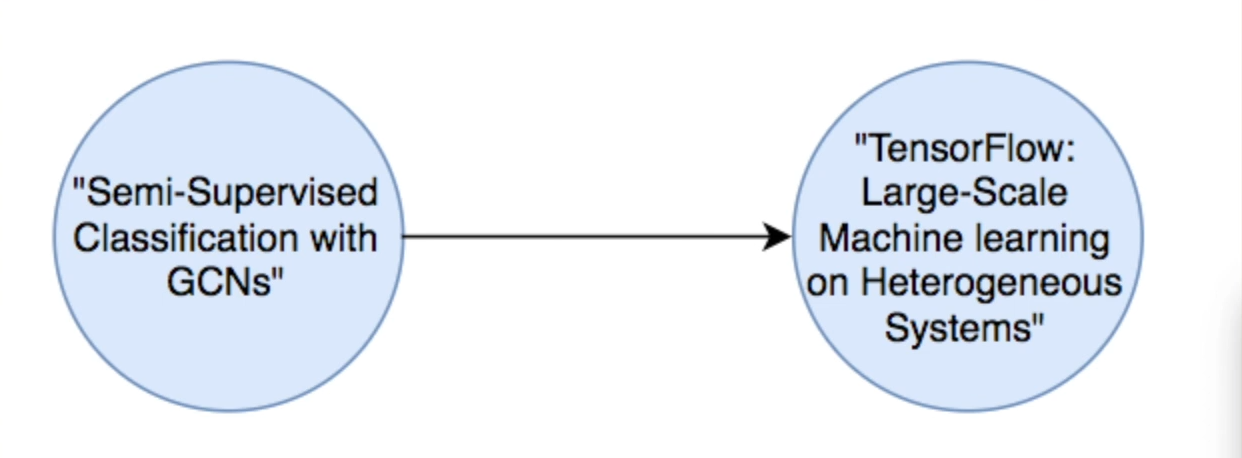
[node of citation Dataset]

The nodes in the dataset might be labelled according to the topic like machine learning on graphs and an edge in the dataset might represent a GCN paper. The citation paper consists of 20 labels per class as in 7 classes would consist of 140 labeled samples.The documents in the citation paper start with [X^0] based on bag of words features.

The initial features in the citation dataset could be understood with the help of GCN propagation rule. We start off with [H(0)] which are the initial features and that could be randomly initialized or could also come from certain graph embeddings such as deep walk. In the case of documents we can use some sort of extra features based on NLP derived metric.

The edges in the dataset when used with gcn are treated as undirected and the reason for this is the limitation which the adjacency matrix has to be symmetric. This problem could be solved by rearranging the directed graphs with bipartite graphs with additional nodes to represent edges.

Conclusion:

Graph convolutional networks are used often in the field of chemistry in which it is used to learn about existing molecular structures and determine new ones. GCNs have also been used for Combinatorial optimization problems.

For further reference, the below paper would be of help:
https://arxiv.org/pdf/1609.02907