
Reading time: 45 minutes
Image denoising is the technique of removing noise or distortions from an image. There are a vast range of application such as blurred images can be made clear. Before going deeper into Image denoising and various image processing techniques, let's first understand:
- What is an Image?
- What is an Image Noise?
- What are the various types of Noise?
Following it, we will understand the various traditional filters and techniques used for image denoising.
What is an Image?
Is it someone's face, a building, an animal, or anything else?
No, An Image is a multidimensional array of numbers ranging from 0 to 255. Each number can be seen as a combination of x(horizontal) and y(vertical) coordinates, called as pixel.
I(x, y) = pixel, where I denotes Intensity at position x and y.
Three different types of Image -
-
Binary image - where pixel value is either 0(dark) or 255(bright).
-
Grayscale image - where pixel value is from range 0 to 255.
-
Color image - Image comprised of 3 channels red(R), green(G) and blue(B). For each channel, pixel value is from range 0 to 255.
Examples of Binary Image, Grayscale Image and Color Image are -

What is an Image Noise?
It is an random variation of brightness or color information in images and an undesirable by-product of image that obscures the desired information.
# Generally, noise is introduced into the image during image transmission, acquisition, coding or processing steps.
Commonly used Noise Models -
Let's Assume -
C(x, y) = Corrupted Noisy Image;
O(x, y) = Original Image;
N(x, y) = Image Noise;
-
Additive Noise - where image noise gets added to original image to produce a corrupted noisy image.
C(x, y) = O(x, y) + N(x, y) -
Multiplicative Noise - where image noise gets multiplied to original image to produce a corrupted noisy image.
C(x, y) = O(x, y) * N(x, y)
What are the various types of Image Noise?
We'll discuss here major four types of noises -
- Gaussian Noise
- Salt and Pepper Noise
- Speckle Noise
- Poisson Noise
1). Gaussian Noise -
It is statistical noise having a probability density function (PDF) equal to that of the Normal Distribution.

Sources -
- During Image Acquisition.
Ex. - sensor noise caused by poor illumination and/or high temperature. - During Transmission.
Ex. - Electronic circuit noise.
2). Salt and Pepper Noise -
Also called Data drop-out.
It is a fixed valued Impulse Noise. This has only two possible values(for 8-bit image), i.e. - 255(bright) for salt noise and 0(dark) for pepper noise.
Sources -
- Sharp and sudden disturbances in the image signal.
- Malfunctioning of camera’s sensor cell.
3). Poisson Noise -
Also called Shot Noise or Quantum(Photon) Noise.
This type of noise has a probability density function of a Poisson distribution.
Source - random fluctuation of photons.
4). Speckle Noise -
Speckle noise is a rough noise that naturally exists in and corrupts the quality of images. Speckle noise can be modeled by multiplying random pixel values with different pixels of an image.
What is Image Denoising?
It is a process to reserve the details of an image while removing the random noise from the image as far as possible.
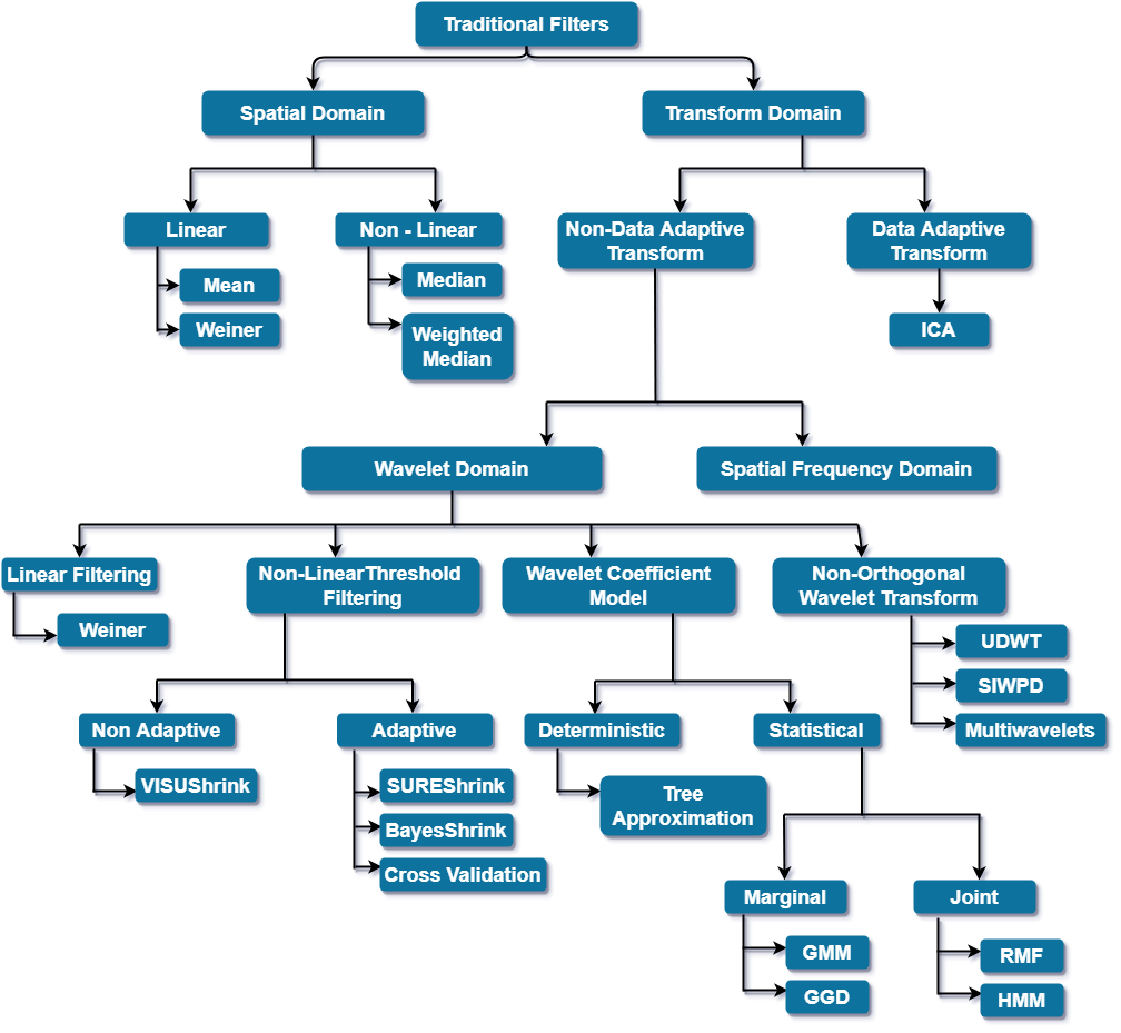
We classify the image denoising filters into 2 broad categories -
1). Traditional Filters - Filters which are traditionally used to remove noise from images. These filters are further divided into Spatial domain filters and Transform domain filters.
2). Fuzzy based Filters - Filters which include the concept of fuzzy logic in their filtering procedure.
In this article we will go through traditional filters in detail.
Let's discuss one by one -
1). Spatial Domain - In this, filters work directly on input image(on pixels of image).
2). Transform Domain - It is needed when it is necessary to analyze the signal. Here, we transform the given signal to another domain and do the denoising procedure there and afterwards inverse of the transformation is done in order to get final output.
Image Denoising Techniques -
1). Spatial Filtering -
It is classified into Linear and Non-Linear filters.
1.1 Linear Filters -
Effective for Gaussian and Salt and Pepper Noise.
1.1.1). Mean Filter -
It is a simple sliding-window filter that replaces the center pixel value in the kernel window with the average (mean) of all the pixel values in that kernel window.
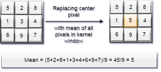
Mean Filter is an optimal filter for gaussian noise in sense of Mean square error.
1.1.2). Weiner Filter -
A statistical approach to remove noise from a signal.
Prerequisite - the user must know the spectral properties(ex. - power functions) of the original signal and noise.
Aim - To have minimum mean-square error(MSE), i.e. the difference between the original signal and the new signal should be as less as possible.
Assume W(x, y) is a weiner filter,
Restored image will be given as -
    Xn(x, y) = W(x, y).Y(x, y)
where,
Y(x, y) is the received image(Degraded).
Xn(x, y) is the restored image.
The equation of Weiner filter obtained while reducing MSE error is -

Where,
- ||H(x, y)||^2 = H(x, y)H*(x, y);
- H(x, y) = degradation function;
- H*(x, y) = complex conjugate of degradation function;
- Sn(x, y) = ||N(x, y)||^2 i.e. Power spectrum of Noise;
- Sf(x, y) = ||F(x, y)||^2 i.e. Power spectrum of undegraded(original) image;
Note - Weiner filter works well only if the underlying signal is smooth.
Drawback of Linear Filter -
Linear filters tend to blur sharp edges, destroy lines and other fine image details, and perform poorly in the presence
of signal-dependent noise.
1.2). Non Linear Filter -
With non-linear filters, the noise is removed without
any attempts to explicitly identify it.
1.2.1). Median Filter -
It is a simple sliding-window filter that replaces the center pixel value in the kernel window with the median of all the pixel values in that kernel window.
Note - The kernel size must be a positive odd integer.
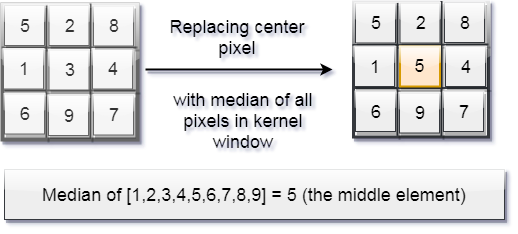
Here, the size is 9, so (9+1)/2 = 5th element is the median.
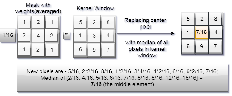
1.2.2). Weighted Median Filter -
Only difference between Median and Weighted Median filter is the presence of Mask. This mask will having some weight (or values) and averaged.
1). This weighted mask is multiply with pixels of kernel window.
2). Pixels are sort into ascending order.
3). Find the median value from the sorted list.
4). Place this median at the centre.
Advantages -
- Can preserve edges.
- Very effective at removing impulsive noise.
- They are more powerful than linear filters because they are able to reduce noise levels without blurring edges.
2). Transform Domain Filtering -
The transform domain filtering methods can be classified according to the choice of the base transformation functions which are Non-Data Adaptive and Data Adaptive filters.
Non-Data Adaptive filters are more popular than Data Adaptive filters.
2.1) Non-Data Adaptive Filters -
Non-Data Adaptive filters are further classified into two domains namely spatial-frequency domain and wavelet
domain.
2.1.1) Spatial Frequency Filtering -
Spatial-frequency filtering refers use of low pass filters
using Fast Fourier Transform (FFT). Here, we predefine a cut-off frequency and this filter passes all the frequencies lower than and attenuates all the frequencies greater than cut-off frequency.
The reason for doing the filtering in the frequency domain is generally because it is computationally faster to perform 2D Fourier transforms and a filter multiply than to perform a convolution in the image (spatial) domain.
Note - Convolution in image(spatial domain) is equivalent to multiplication in frequency domain.
2.1.2) Wavelet Domain -
A wavelet is a mathematical function used to divide a given function or continuous-time signal into different scale components.
A wavelet transform is the representation of a function by wavelets. Filtering methods in wavelet domain are further classified into -
2.1.2.1) Linear Filters -
Weiner filter yield optimal results when there is Gaussian based noise and the accuracy criterion is the mean square error (MSE).
However, designing a filter based on this assumption results into displeasing results.
2.1.2.2) Non Linear Threshold Filtering -
Why thresholding is effective in noise reduction?
Because fo these following assumptions -
- The decorrelating property of a wavelet transform creates a sparse signal: most untouched coefficients are zero or close to zero.
- Noise is spread out equally along all coefficients.
- The noise level is not too high so that we can distinguish the signal wavelet coefficients from the noisy ones.
There are two types of Thresholding - Hard and Soft.
1). Hard Thresholding - is a “keep or kill” procedure and
is more intuitively appealing.
The hard thresholding operator with threshold t is defined as -
D(U, t) = U for all |U| > t
        = 0 otherwise
2). Soft Thresholding - shrinks coefficients above the threshold in absolute value.
The soft thresholding operator with threshold t is defined as -
D(U, t) = sgn(U)max(0, |U| - t)
Advantage of Soft thresholding over Hard thresholding -
Sometimes, pure noise coefficients may pass the hard threshold and appear as annoying 'blips' in the output. Soft thesholding shrinks these false structures.
The difference between various threshold filtering techniques is only of threshold selection, the basic procedure of threshold filtering remains the same : -
- Calculate the Discrete wavelet transform(DWT) of the image.
- Threshold the wavelet coefficients.(Threshold
may be universal or subband adaptive) - Compute the Inverse DWT to get the denoised estimate.
Now, come to it's types - Adaptive and Non Adaptive.
- Non Adaptive: VisuShrink;
- Adaptive - SUREShrink, BayesShrink, Cross Validation;
1). VisuShrink -
This approach employs a single, universal threshold to all wavelet detail coefficients.
The value of this universal threshold(ut) is -
Where,
σ = Noise variance;- M = Total number of pixels in the image.
This threshold is designed to remove additive Gaussian noise with high probability, which tends to result in overly smooth image appearance.
Why VisuShrink is non adaptive in nature ?
Since, the ut tends to be high(because of it's constraint that with high probability the estimate should be at least as smooth as the signal) for large values of M, so, it kills many signal coefficients along with the noise. Thus, the threshold does not adapt well to discontinuities in the signal.
2). SUREShrink -
SURE - Stein's unbiased Risk Estimate.
SUREShrink is a smoothness-adaptive hybrid scheme, it consists of two threshold values. We use -
- Universal threshold, for sparse situations.
- The threshold that minimizes SURE, for dense situations.
SureShrink is subband adaptive technique - a separate threshold is computed for each detail subband.
# Why there are two thresholds in this technique?
In case of extreme sparsity of the wavelet coefficients, the noise contributed to the SURE profile by many coordinates(where the signal is zero) destroys the information contributed to the SURE profile by the few coordinates(where the signal is non-zero).
Therefore, SURE principle has drawback in situations of extreme sparsity of the wavelet coefficients, and so we use universal threshold for these situations.
Advantages of SUREShrink over VisuShrink -
The sharp features of the original image are retained in restored image and the MSE is lower than that of VisuShrink.
3). BayesShrink -
BayesShrink is an Adaptive technique, here we determine the threshold for each subband.
Here, for each subband we assume a Generalized Gaussian
Distribution(GGD).
The value of data-driven, subband-dependent threshold used in BayesShrink is -
Where,
Advantages of BayesShrink over SureShrink -
- BayesShrink performs better than SureShrink in terms of MSE.
- The reconstruction using BayesShrink is smoother and more visually appealing than the one obtained using SureShrink.
4). Cross Validation -
Cross Validation replaces wavelet coefficient with the weighted average of neighborhood coefficients to minimize generalized cross validation (GCV) function providing optimum threshold for every coefficient.
2.1.2.3) Wavelet Coefficient Model -
This approach focuses on exploiting the multiresolution properties of Wavelet Transform. This technique identifies close correlation of signal at different resolutions by observing the signal across multiple resolutions.
Note - This method is computationally much more complex and expensive, but produces Excellent output .
The modeling of the wavelet coefficients can either be deterministic or statistical.
1). Deterministic -
The Deterministic method of modeling involves creating tree structure of wavelet coefficients.
Here, in this tree -
1). Each level represents each scale of transformation.
2). Each node represent the particular wavelet coefficient.
The optimal tree approximation displays a hierarchical interpretation of wavelet decomposition.
Note -
- If a wavelet coefficient has strong presence at particular node then in case of it being signal, it's presence should be more pronounced at its parent nodes.
- If it is noisy coefficient, for instance spurious blip, then such consistent presence will be missing.
2). Statistical -
This approach focuses on interesting and appealing properties of the Wavelet Transform such as -
1). multi-scale correlation between the wavelet coefficients.
2). local correlation between neighborhood coefficients etc.
This approach has an inherent goal of perfecting the exact modeling of image data with use of Wavelet Transform.
There are two techniques to perform statistical modeling of wvelet transform -
a). Marginal Probabilistic Model -
The marginal distributions of wavelet coefficients usually have a marked peak at zero and heavy tails.
The commonly used methods to model the wavelet coefficients
distribution are -
1). GMM - Gaussian Mixture Model, simpler to use.
2). GGD - Generalized Gaussian Distribution, produce more accurate results.
b). Joint Probabilistic Model -
The commonly used methods to model the wavelet coefficients distribution are -
1). HMM - Hidden Markov Model, used to capture intra-scale correlations. Once the correlation is captured by HMM, Expectation Maximization is used to estimate the required parameters and from those, denoised signal is estimated from noisy observation using well known MAP(Maximum A Posteriori) estimator.
2). RMF - Random Markov Field, used to capture inter-scale correlations.
The complexity of local structures is not well described by Random Markov Gaussian densities whereas Hidden Markov Models can be used to capture higher order statistics.
2.1.2.4) Non-orthogonal Wavelet Transforms -
What is Orthogonal Wavelet?
-> Whose inverse wavelet transform is the adjoint of the wavelet transform.
Of course, non-orthogonal wavelet is opposite of orthogonal wavelet.
3 Techniques are there -
1). Undecimated Wavelet Transform (UDWT) - a shift invariant technique, used for decomposing the signal to provide visually better solution. It avoids visual artifacts such as pseudo-Gibbs phenomenon. Though results are quite good but UDWT is less feasible as it adds a large overhead of computations.
2). Shift Invariant Wavelet Packet Decomposition (SIWPD) is exploited to obtain number of basis functions. Then using Minimum Description Length principle the best basis function is found out which yielded smallest code length required for description of the given data. Then, thresholding was applied to denoise the data.
3). Multiwavelets outperforms UDWT in performance but further increases the computation complexity. The multiwavelets are obtained by applying more than one mother function (scaling function) to given DWT of image. Multiwavelets possess properties such as short support, symmetry, and the most importantly higher order of vanishing moments.
2.2) Data Adaptive Transform -
Independent Component Analysis (ICA) -
"Independent component analysis (ICA) is a method for finding underlying factors or components from multivariate (multi-dimensional) statistical data. What distinguishes ICA from other methods is that it looks for components that are both statistically independent, and nonGaussian."
-A.Hyvarinen, A.Karhunen, E.Oja
Read more about Independent Component Analysis (ICA)Assumption - Non-Gaussian Signal.
This assumption helps the algorithm to denoise images with Non-Gaussian and Gaussian distribution both.
Drawbacks as compared to wavelet based methods are:
- the computational cost because it uses a sliding
window. - it requires sample of noise free data or at least two image frames of the same scene. In some applications, it might be difficult to obtain the noise free training data.
Besides all these techniques, there is one more technique:
- Denoising Autoencoders, used to remove noise from images, about which we have already discuss in my another article "Applications of Autoencoders".