Importance of Loss Function in Machine Learning

Reading time: 25 minutes

Assume you are given a task to fill a bag with 10 Kg of sand. You fill it up till the measuring machine gives you a perfect reading of 10 Kg or you take out the sand if the reading exceeds 10kg.

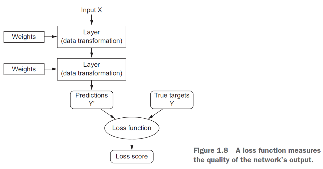
Just like that weighing machine, if your predictions are off, your loss function will output a higher number. If they’re pretty good, it’ll output a lower number. As you experiment with your algorithm to try and improve your model, your loss function will tell you if you’re getting(or reaching) anywhere.

"The function we want to minimize or maximize is called the objective function or criterion. When we are minimizing it, we may also call it the cost function, loss function, or error function" - Source

At its core, a loss function is a measure of how good your prediction model does in terms of being able to predict the expected outcome(or value). We convert the learning problem into an optimization problem, define a loss function and then optimize the algorithm to minimize the loss function.

What are the types of loss functions?

**Most commonly used loss functions are:

• Mean Squared error

• Mean Absolute Error

• Log-Likelihood Loss

• Hinge Loss

• Huber Loss

• Mean Squared Error

Mean Squared Error (MSE) is the workspace of basic loss functions, as it is easy to understand and implement and generally works pretty well. To calculate MSE, you take the difference between your model's predictions and the ground truth, square it out and then average it out across the whole dataset.
The result is always positive regardless of the sign of the predicted and ground truth values and a perfect value is 0.0.

# function to calculate MSE
def MSE(y_predicted, y_actual):

    squared_error = (y_predicted - y_actual) ** 2
    sum_squared_error = np.sum(squared_error)
    mse = sum_squared_error / y_actual.size

    return mse

• Mean Absolute Error

Mean Absolute Error (MAE) is only slightly different in definition from the MSE, but interestingly provides almost exactly opposite properties. To calculate the MAE, you take the difference between your model’s predictions and the ground truth, apply the absolute value to that difference, and then average it out across the whole dataset.

# function to calculate MAE
def MAE(y_predicted, y_actual):
    
    abs_error = np.abs(y_predicted - y_actual)
    sum_abs_error = np.sum(abs_error)
    mae = sum_abs_error / y_actual.size
    
    return mae

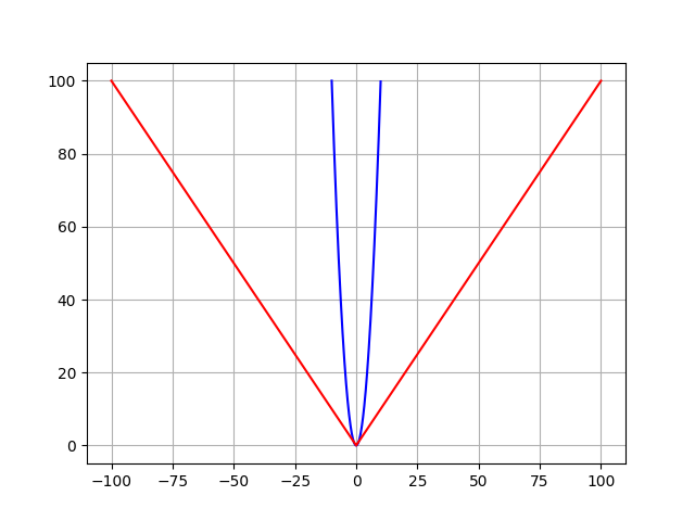
MSE (blue) and MAE (red) loss functions.

• Log-Likelihood Loss

This loss function is also relatively simple and commonly used in classification problems. In this,
the error between two probability distributions is measured using cross-entropy.

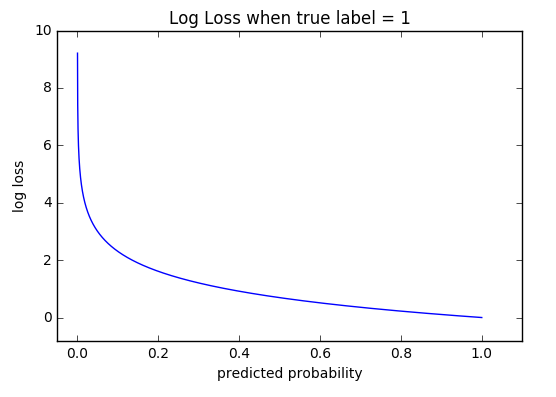
-(y_actual * log(y_predicted) + (1 - y_actual) * log(1 - y_predicted))

Here, you can see that when the actual class is 1, the second half of the function disappears, and when the actual class is 0, the first half drops. That way, we just end up multiplying the log of the actual predicted probability for the ground truth class.

Source: fast.ai

Cross-entropy for a binary or two-class prediction problem is actually calculated as the average cross-entropy across all examples.

from math import log
 
# function to calculate binary cross entropy
def binary_cross_entropy(actual, predicted):
	sum_score = 0.0
	for i in range(len(actual)):
		sum_score += actual[i] * log(1e-15 + predicted[i])
	mean_sum_score = 1.0 / len(actual) * sum_score
	return -mean_sum_score

This function is one of the most popular measures for Kaggle competitions. It's just a straightforward modification of the likelihood function with logarithms.

• Hinge Loss

The Hinge loss function is popular with Support Vector Machines(SVMs). These are used for training the classifiers. Let 't' be the target output such that t = -1 or 1, and the classifier score be 'y', then the hinge loss for the prediction is given as: L(y) = max(0, 1-t.y)

• Huber Loss

We know that MSE is great for learning outliers while the MAE is great for ignoring them. But what about something in the middle?
Consider an example where we have a dataset of 100 values we would like our model to be trained to predict. Out of all that data, 25% of the expected values are 5 while the other 75% is 10.

An MSE loss wouldn’t quite do the trick since we don’t have “outliers”; 25% is by no means a small fraction. On the other hand, we don’t necessarily want to weight that 25% too low with an MAE. Those values of 5 aren’t close to the median (10 — since 75% of the points have a value of 10), but they’re also not outliers.

Our solution?

The Huber Loss Function.

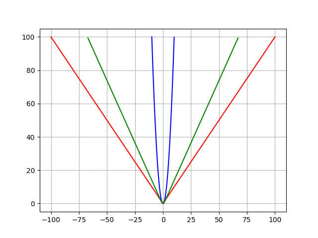
The Huber Loss offers the best of both worlds by balancing the MSE and MAE together. We can define it using the following piecewise function:

What this equation actually means is that for loss values less than delta, use the MSE; for loss values greater than delta, use the MAE. This effectively combines the best of both worlds from the two loss functions.

# function to calculate Huber loss
def huber_loss(y_predicted, y_actual, delta=1.0):

    huber_mse = 0.5*(y_actual-y_predicted)**2
    huber_mae = delta * (np.abs(y_actual - y_predicted) - 0.5 * delta)
    
    return np.where(np.abs(y_actual - y_predicted) <= delta, 
                             huber_mse,  huber_mae)

MSE (blue), MAE (red) and Huber (green) loss functions.

Conclusion

Loss functions provide more than just a static representation of how your model is performing–they’re how your algorithms fit data in the first place. Most machine learning algorithms use some sort of loss function in the process of optimization or finding the best parameters (weights) for your data.

Importantly, the choice of the loss function is directly related to the activation function used in the output layer of your neural network. These two design elements are connected.

Think of the configuration of the output layer as a choice about the framing of your prediction problem, and the choice of the loss function as the way to calculate the error for a given framing of your problem.

Further reading
Deep Learning Book by Ian Goodfellow, Yoshua Bengio and Aaron Courville.