Intuitive Introduction to Gaussian Processes

Reading time: 30 minutes | Coding time: 10 minutes

A Gaussian Process is a non-parametric model that can be used to represent a distribution over functions.

Lets break this definition down.

What does it mean for a model to be parametric or non-parametric?

Parametric models

Parametric models assume that the data distribution (set of input points, images etc.) can be entirely defined in terms of a finite set of parameters theta. For example in simple linear regression the parameters are the m and c in the equation y = mx + c.

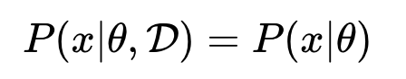
Such that if the model is given the parameters, a future prediction is independent of the data. This is exemplified in the image below where x is the future predictions, parameter is theta, and D is the observed data.

This implies that the finite set of parameters captures everything you need to know about the data. Even if the amount of data is unbounded the complexity of model is bounded this makes parametric models not very flexible

Some examples of these models are polynomial regression, logistic regression, and mixture models.

I like to remember this by imagining a parametric model as a person who is complacent and arrogant. Despite what new information you present them they will always come to the same conclusion because their mindset is fixed.

Non-parametric models

These are models that assume that the data distribution cannot be defined in terms of a finite set of parameters.

These type of models are usually defined by assuming an infinite dimensional
theta, that we can look at as a function (I'll explain more further down).

By doing this the amount of information that theta is able to capture from the data D can grow as the amount of data grows. Making these types of models way more flexible than parametric models.

A Gaussian process (GP) is one of these models.
They are cool because they allows us to:

• Model any black box function
• Model uncertainty (Valuable in situations where confidence matters such as health-care)

So now we know what it means for GPs to be non-parametric now we're going to look at how functions are modeled using Gaussians.

Modeling functions using Gaussians

Key Idea: Any function can be modeled by an infinite dimensional multivariate Gaussian Distribution

This is such a confusing statement, it is just begging to be unpacked.

Basics of the Gaussian

A good first step is to look at what a Gaussian distribution is and what it means.

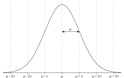
Many of you will be extremely familiar with the bell curve shape of the normal distribution shown below.

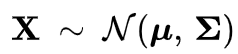
As well as it's equation, the one shown below is the multivariate Gaussian distribution equation. Where mu is the mean and sigma is the covariance matrix.

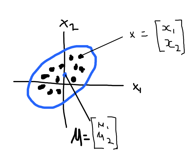
Gaussians are usually used to describe any set of correlated random variables that cluster around a mean. In my crude drawing below the blue represents a 2D Gaussian. The blue dot represents the mean (roughly) where the Gaussian in centered. I didn't give the value for sigma but the covariance matrix here just describes how each random variable varies in relation to each other random variables.

So now we have some idea about what makes up a Gaussian let's see how we can use a Gaussian to get some points and then eventually a function.

How do we get points or functions from a Gaussian?

Once we have built our Gaussian by defining the mean and the covariance matrix we can use it to produce data (a.k.a draw samples).

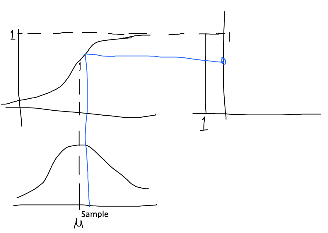
A common technique is inverse CDF sampling. If we know the cumulative distribution function (CDF) of the distribution we can generate a random sample. Verfy briefly what happens is you generate a random (uniformly distributed) number between 0 and 1 and you use this with the inverse cdf to get a value from the Gaussian distribution. Once again I show this below in my crude illustration.

So now you might be saying "What does this have to do with functions!!!".

If we have a 2D Gaussian and we sample it using the trick we just learned we get 2 points. We can plot these 2 points and join them up in order and form a line. You can do this as many times as you like. In the image below from (http://bridg.land/posts/gaussian-processes-1) they sampled the Gaussian 10 times to get 10 lines.

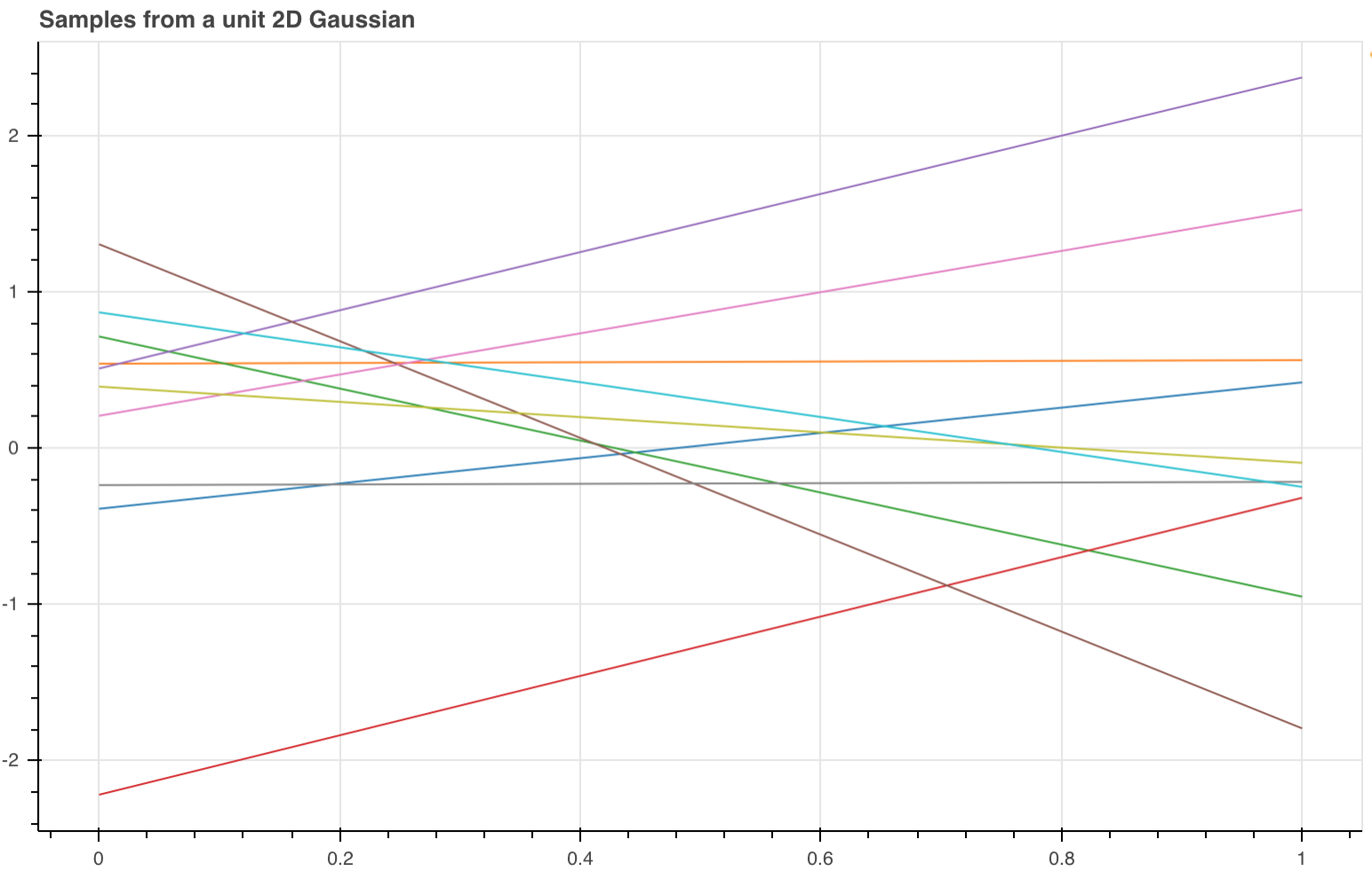
The key fact here is that for an N-D Gaussian if you sample it once you get N-points.

So if you sample a 3D Gaussian you get 3 points, a 30D Gaussian you get 30 points and if you sample an infinite dimensional Gaussian you get an infinite number of points.

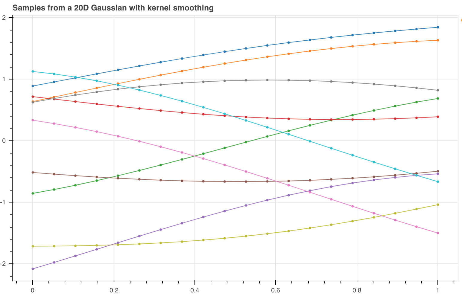
The image below shows 10 samples form a 20D Gaussian.

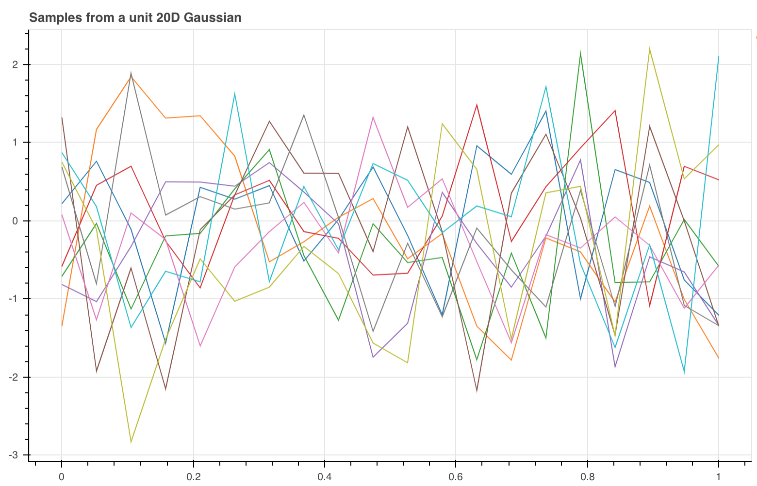
As the number of dimensions gets closer to infinity it means that we do not have to join up the points because we will have a point for every possible input.

To draw samples from a GP you provide the mean and covariance and all the magic happens. Don't be worried that this is slightly different than before. It is because in the case below we are drawing a sample from a multivariate Gaussian distribution (MVG). The idea is still the same, we can generates points and append it to make a sampled vector. You use a decomposition because it allows us to get something akin the sqrt of a matrix so that we can express our MVG as transformation of a unit MVG.

def draw_samples(self, mean, covariance, num_samples=1):
    # Every time we sample a D dimensional gaussian we get D points 
    all_samples = []

    # SVD gives better numerical stability than Cholesky Decomp (it was giving errors)
    num_dimensions = len(mean)

    for _ in range(0, num_samples):
        z = np.random.standard_normal(num_dimensions)

        [U, S, V] = np.linalg.svd(covariance)
        A = U * np.sqrt(S)

        all_samples.append(mean + np.dot(A, z))

    return all_samples

A point for every possible input sounds a lot like a function to me.

But these graphs are really noisy. This is because in these graphs they haven't imposed any constraints on how similar the points are.

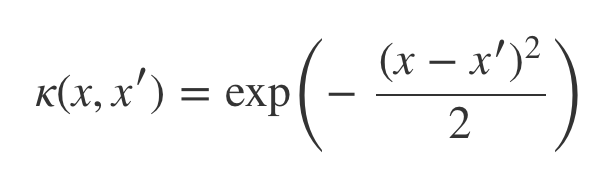
To smooth the functions (lines above) we need a measure of similarity called the squared exponential kernel (image below) . According to this function if two input points are equal then its value is 1 otherwise it tends to 0 the further apart they get.

def kernel(self, a, b):
    # Squared Exponential Kernel Function for GP
    square_distance = np.sum((a - b) ** 2)
    return np.exp(-0.5 * square_distance)

Populating a covariance matrix of a Gaussian using the kernel function means that when you perform the sample points should not vary much between each other if they are close in space. Producing lines that look better (see image below) however this doesn't tell us how to actually model a function.

In this section we have seen that it is possible to sample a Gaussian to get functions, making the Gaussian Process a distribution over functions.

Modeling a function

Let's assume there is a function we are trying to model given a whole bunch of data from this secret function.

How do we train a GP?
We have the data points, the x's and we use this to construct the covariance matrix which describes the relationship between the given data points. But it is important to remember that the distribution is over the labels, the y's.

def train(self):
    # GP training means constructing K
    mean = np.zeros(len(self.train_x))
    covariance = self.build_covariance(self.train_x, self.train_x)

    return mean, covariance

What about when we want to predict the labels y* for some new set of data x* ?

This is when it starts to get tricky because we need to go from a joint distribution to a conditional distribution.

Why? Because the way the MV Gaussian Distribution is defined, is as a joint distribution.

To get closer, we can do a trick and add the new y* and x* to the definition but that only models p(y, y*| x , x*).

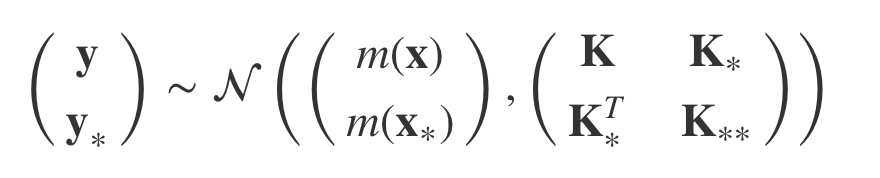
But we want p(y* | x, y, x*). How do we get it ?

We need to condition the multivariate Gaussian on y* because we only want a distribution over y*. Fortunately for us someone has already gone through all of the work of figuring out how to do this. It tells us how to update the mean and the covariance such that we predict y* given x* and our training data (x and y).

def _predict(self, covariance_k):
    k = covariance_k
    k_star = self.build_covariance(self.train_x, self.test_x)
    k_star_star = self.build_covariance(self.test_x, self.test_x)

    k_star_inv = k_star.T.dot(np.linalg.pinv(k))
    mu_s = k_star_inv.dot(self.train_y)
    sigma_s = k_star_star - np.matmul(k_star_inv, k_star)
    return (mu_s, sigma_s)

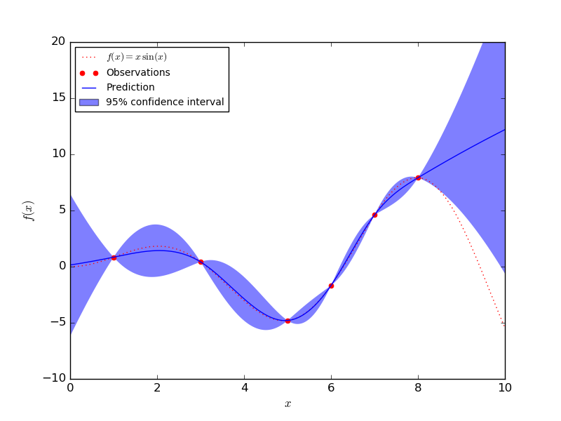
The new mean tells us what the y* value is and the new variance gives us to get a confident measurement. We can use this new mean and covariance to sample functions. As well as a function for the points we also get a function for the upper and lower confidence bounds.

An example result from Scikit-learn can be seen below. As you get near the data points (observations) the uncertainty gets smaller. The observations bind any predicted function to that region.

Complexity of Gaussian Processes

For a dataset of size N the complexities are as follows:
Time complexity: Θ(N^3)
Space complexity: Θ(N^2)

Gaussian processes are very powerful but due to the large time complexities it is unfortunately not feasible to use them in many real world applications.

All of the code in this post can be found in my GitHub repository found here.

Resources
Introduction to Gaussian Processes
Introduction to Gaussian processes by Nando De Freitas