Laplacian Filter (also known as Laplacian over Gaussian Filter (LoG)), in Machine Learning, is a convolution filter used in the convolution layer to detect edges in input.

Ever thought how the computer extracts a particular object from the scenery. How exactly we can differentiate between the object of interest and background.
Well a simple baseline answer could be: Edge Detection.

Before diving into the mechanics of it, let’s understand why specifically edge detection.

Try and look around you and find any object of your choice. It may be a book, apple or anything within your sight. Now, see the shape of that object.

Ask yourself, how did you figure out the shape of that particular object? Well, internally you are doing a subtraction. Subtraction of the object from its surroundings. That’s how you can say that, this is the shape. Not only that, if you were not able to distinguish that then you won’t even know that there is an object or not. What happens when you place a black book in front of black box? You won’t know there is anything, especially if they resonate the same colors.

Hence, in identifying the object, the first step is to separate it from the background. And to put it into technical terms: to detect the edge of the object.
Now, that you have an incentive to learn the topic, let’s start.

Laplacian filter is something that can help you with edge detection in your applications.

Laplacian filters are derivative filters used to extract the vertical as well as horizontal edges from an image. This is how they separate themselves from the usual sobel filters.

Sobel filters are single derivative filters, that means that they can only find edges in a single dimension.

Why are they called derivative? And how exactly are we going to get the edges?

Wait, we will explain it all. The thing is that how can you detect and edge exactly? You find a difference between the borders and hence you say that this is one object and that is another. For example, if you have a green book placed on a blue table, then the color change from blue to green denotes a change of object. Hence, draws a line separating book from the table.

To put it technically we are checking for a change in pixel intensities, as we always work on grayscale images and the best way to see different colors on a grayscale is to check the pixel intensities.

So, if there is a bump in the pixel intensity, we can say that there is an edge.
Now to detect an edge we need to do it mathematically. To do so we can take a derivative of intensity and hence can find a bump in intensity wherever it exists and that is how we find the answer.

This is how sobel filters work. They take one derivative and find an edge in either of the one dimension (x or y).
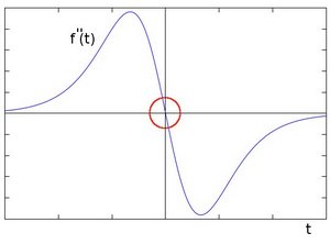
But with Laplacian filter, we can get edges in both dimensions, hence we take double derivative of the intensities. And what happens when we do double derivation, the graph points to zero. So we will check those pixels which lead to zero and then mark them as edge points. The reference graph (Credit: OpenCV.org) is as follows:

Some of the most common filters used to create the laplacian are:

First

0	1	0
1	-4	1
0	1	0

Second

-1	-1	-1
-1	8	-1
-1	-1	-1

Both of these are created by the following equation. As we discussed we need double derviation of every pixel, so that we can check the pixel intensities.

Now as we are clear with the theory, let’s look at the actual steps.

One thing to note is that the Laplacian filter is a bit too sensitive. So, it will work badly if there is noise in the image. Hence we apply something known as a Gaussian Blur to smooth the image and make the Laplacian filter more effective.

Note: Due to this addition of the gaussian filter, the overall filter is always in a pair. And in normal dialogues you may hear Laplacian over the Gaussian Filter (LoG). Which shouldn’t be confused as another filter, but just that it comes with the Gaussian blur, nothing else.

Now, let's break down the Laplacian as well as the Gaussian blur functions and implement our own functions.

Steps:

• We will define a function for the filter
• Then we will make the mask
• Then we will define function to iterate that filter over the image(mask)
• We will make a function for checking the zeros as explained
• And finally a function to bind all this together

One thing to keep in mind is that to create a combination of the filters, i.e. Laplacian over gaussian filter (LoG), then we can use the following formula to combine both of them.

Following is the function to define the above equation:

def l_o_g(x, y, sigma):
    # Formatted this way for readability
    nom = ( (y**2)+(x**2)-2*(sigma**2) )
    denom = ( (2*math.pi*(sigma**6) ))
    expo = math.exp( -((x**2)+(y**2))/(2*(sigma**2)) )
    return nom*expo/denom

Note: Don't be confused by the equation and the code being abit different. But the code has been written for the simplified equation (which can be found by compounding the inner subtraction as well as multiplication of outer denominator).

As we are breaking down the filter, we would also need some additional functions. Those are:

• A function to take the filter and convolve around the image.
• A function for creating the actual mask.
• And finally a function to check the zeros.

Function(s) logic:

Create_log fucntion:

1. Calculate w by using the size of filter and sigma value
2. Check if it is even of not, if it even make it odd, by adding 1
3. Iterate through the pixels and apply log filter and then append those changed pixels into a new array, and then reshape the array.

Convolve function:

1. Extract the heights and width of the image
2. Now make a range of pixels which are covered by the mask (output of filter)
3. Make an array of zeros (res_image)
4. Now iterate through the image and append the values of product of mask and the original image and append it to the res_image array.

Zeros function (To mark the edges):

1. Make a zeros array of same dimensions of the log_image (zc_image)
2. Now iterate over the image and check two values, if they are equal to zero or not. If they are not equal to zero then check if values are positive or negative.
   If the pixel value is zero, that means there an edge exist.
   If none of the pixels, are zero, that means there is no edge.
3. Now whichever pixels were zero, append those coordinates to zc_image array.
4. Make all the pixels in zc_image as 1, meaning white. That will show the edges.

Now that we understand the logic of coding the functions, let us see how we can implement them in Python.

Creating the filter image:

def create_log(sigma, size = 7):
    w = math.ceil(float(size)*float(sigma))

    if(w%2 == 0):
        w = w + 1

    l_o_g_mask = []

    w_range = int(math.floor(w/2))
    print("Going from " + str(-w_range) + " to " + str(w_range))
    for i in range_inc(-w_range, w_range):
        for j in range_inc(-w_range, w_range):
            l_o_g_mask.append(l_o_g(i,j,sigma))
    l_o_g_mask = np.array(l_o_g_mask)
    l_o_g_mask = l_o_g_mask.reshape(w,w)
    return l_o_g_mask

Convolving the filter over the original image

def convolve(image, mask):
    width = image.shape[1]
    height = image.shape[0]
    w_range = int(math.floor(mask.shape[0]/2))

    res_image = np.zeros((height, width))

    # Iterate over every pixel that can be covered by the mask
    for i in range(w_range,width-w_range):
        for j in range(w_range,height-w_range):
            # Then convolute with the mask 
            for k in range_inc(-w_range,w_range):
                for h in range_inc(-w_range,w_range):
                    res_image[j, i] += mask[w_range+h,w_range+k]*image[j+h,i+k]
    return res_image

Checking the zeros to mark the edges

def z_c_test(l_o_g_image):
    z_c_image = np.zeros(l_o_g_image.shape)

    # Check the sign (negative or positive) of all the pixels around each pixel
    for i in range(1,l_o_g_image.shape[0]-1):
        for j in range(1,l_o_g_image.shape[1]-1):
            neg_count = 0
            pos_count = 0
            for a in range_inc(-1, 1):
                for b in range_inc(-1,1):
                    if(a != 0 and b != 0):
                        if(l_o_g_image[i+a,j+b] < 0):
                            neg_count += 1
                        elif(l_o_g_image[i+a,j+b] > 0):
                            pos_count += 1

            # If all the signs around the pixel are the same and they're not all zero, then it's not a zero crossing and not an edge. 
            # Otherwise, copy it to the edge map.
            z_c = ( (neg_count > 0) and (pos_count > 0) )
            if(z_c):
                z_c_image[i,j] = 1

    return z_c_image

And this is how we put it all together, to finally generate the image. Do note, we need to pass a grayscale image in the final function, not the original one.
So we will make one final function to take in the image and given the sigma value, generate the masked image.

def run_l_o_g(bin_image, sigma_val, size_val):
    # Create the l_o_g mask
    print("creating mask")
    l_o_g_mask = create_log(sigma_val, size_val)

    # Smooth the image by convolving with the LoG mask
    print("smoothing")
    l_o_g_image = convolve(bin_image, l_o_g_mask)

    # Display the smoothed imgage
    blurred = fig.add_subplot(1,4,2)
    blurred.imshow(l_o_g_image, cmap=cm.gray)

    # Find the zero crossings
    print("finding zero crossings")
    z_c_image = z_c_test(l_o_g_image)
    print(z_c_image)

    #Display the zero crossings
    edges = fig.add_subplot(1,4,3)
    edges.imshow(z_c_image, cmap=cm.gray)
    pylab.show()

And finally you may experiment with other values of sigma, and see the changes in intensities.

If this seems like too much work, we can also implement it using the OpenCv library and the in-built functions. This is how we can implement it in Python.

OpenCV Implementation

Steps:

• Load the image.
• Remove the noise by applying the Gaussian Blur.
• Convert the image into grayscale.
• Apply Laplacian Filter.
• See the output.

We will use the OpenCV library to code this in. We will also implement the filters from scratch. The code for the same is followed after the base code.

Code:

Import the libraries:

import cv2
import matplotlib.pyplot as plt

Load the image:

source = cv2.imread('WallpaperStudio10-62073.jpg', cv2.IMREAD_COLOR)

Here the first argument is to define the path of the image and second defines how you want to read the image. Here we want to read the image in color hence we use IMREAD_COLOR.

Image loaded is:

Remove noise by applying Gaussian Blur:

source = cv2.GaussianBlur(source, (3, 3), 0)

Here, first argument is the image. Second defines the kernel size.

Convert to grayscale:

source_gray = cv2.cvtColor(source, cv2.COLOR_BGR2GRAY)

Apply the Laplacian Filter:

dest = cv2.Laplacian(source_gray, cv2.CV_16S, ksize=3)
abs_dest = cv2.convertScaleAbs(dest)

Show the output:

plt.imshow(abs_dst, cmap="gray")

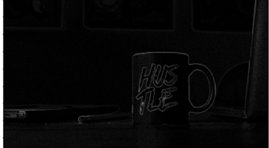
Now you can see the Laplacian filter gets the mug edges clearly and also takes in the internal text on the mug.

Pretty decent right? This is how you can apply an edge detector by using Laplacian or Laplacian over Gaussian filter. With this article at OpenGenus, you must have the complete idea of Laplacian Filter. Enjoy.