In this article, we will implement a Naive Bayes classifier from scratch to perform sentiment analysis.

Table of Contents

• Overview of Sentiment Analysis
• Overview of Bayes' Theorem and How it Applies to Sentiment Analysis
• Overview of Naive Bayes for Sentiment Analysis
• Dataset
• Installation and Setup
• Calculating Word Frequency
• Calculating Probabilities and Implementing the Classifier
• Testing and Results
• Conclusion

Overview of Sentiment Analysis

Sentiment Analysis is the process of classifying whether textual data is positive, negative, or neutral. Some use cases of sentiment analysis include:

• Monitoring product feedback by determining whether customers' opinions are positive, neutral, or negative.
• Targeting people to improve their service. Businesses can reach out to customers who feel negatively about a product.
• Gauging opinions on social media about a particular issue.

In this article, we will be learning the mathematics behind a machine learning algorithm called Naive Bayes. We will then implement it from scratch to perform sentiment analysis.

Overview of Bayes' Theorem and How it Applies to Sentiment Analysis

Naive Bayes is a supervised machine learning algorithm based on Bayes’ theorem. Bayes' theorem is defined mathematically as the following equation:

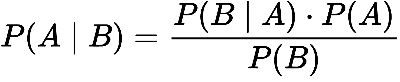
• P(A|B) represents the probability of event A happening given that B is true.
• P(B|A) represents the probability of event B happening given that A is true.
• P(A) and P(B) are the probabilities of observing A and B without any prior conditions. These are referred to as prior probabilities.

Imagine we are trying to classify the sentence "I like this article" as either positive or negative. We would first determine the probability that the text is positive and the probability that the text is negative. We would then compare the two probabilities. To calculate the probability of "I like this article" being positive, we can rewrite Bayes' theorem as follows (we would do the same thing for the negative class, except we would replace all occurrences of "Positive" with "Negative"):

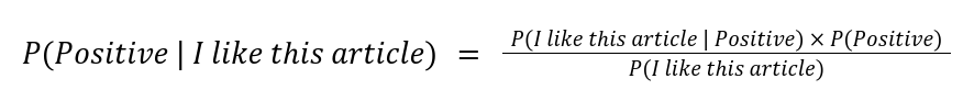
• P(Positive | I like this article) represents the probability of the text "I like this article" being positive.
• P(I like this article | Positive) represents the probability of a positive text being "I like this article". To calculate this, we can count the number of occurrences of "I like this article" in the positive texts and divide it by the total number of samples labeled as positive.
• P(Positive) is the prior probability of a training sample being classified as positive. For example, if there are 10 sentences in our training data, and 7 sentences are positive, then P(Positive) would be 7/10.
• We can discard the denominator since the denominator will be the same for each class.

Overview of Naive Bayes for Sentiment Analysis

Based on our current formula, P(I like this article | Positive) would return 0 if there are no exact matches of "I like this article" in the positive category from the training dataset. Our model won't be very useful if sentences that we can only correctly classify those sentences that appear in the training data. This is where the "Naive" part of Naive Bayes comes into play.

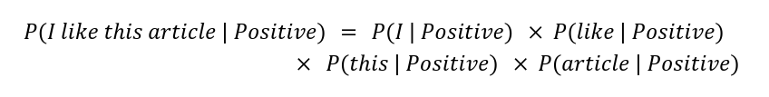
Naive Bayes assumes that every word in the sentence is independent of the other words. Context does not matter. The sentence "I like this article" and "this article I like" are the same for a Naive Bayes classifier. Instead of counting the occurrences of specific sentences in the training data, we are now looking at the frequency of individual words. The below equation demonstrates how we can calculate P (I like this article | Positive):

Calculating P(like | Positive) is done by dividing the number of occurrences "like" appears in positive texts divided by the total number of words in positive texts. For example, if there are 3 occurrences of "like" in positive texts and there are 11 total words, P(like | Positive) would be calculated as follows:

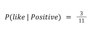
This same method is used for every word and class.

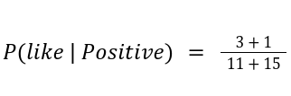
However, what if "like" did not appear even once in the training data? That would cause P(like | Positive) to be 0. Since we multiply this probability by all the others, we will end up with an overall probability of 0. This doesn't give us any relevant information. To fix this, we apply Laplace smoothing to each individual word's probability.

In Laplace smoothing, we add 1 to the numerator to ensure that the probability won't be 0. To prevent the probability from being greater than 100%, we add the total number of possible words to the divisor. For example, if there were 15 unique words that appeared in the training data (regardless of the label), we would add 15 to the denominator. The equation below demonstrates this:

After calculating all the individual word probabilities and applying Laplace smoothing to each of them, we finally multiply them together. We multiply the result by the prior probability of the class. After that, all we do is compare which class has the greatest probability; this class is the output of the classifier.

Implementation

Now, we will go over an implementation of a Naive Bayes classifier from scratch in Python.

Dataset

We will be using the IMDb movie reviews dataset. You can download this dataset in CSV format using this link. Please see this link for more information.

When you download it, rename the file to imdb_reviews.csv.

Installation and Setup

The only library we will be using is The Natural Language Toolkit (NLTK) for text preprocessing (tokenization, removing stop words, lemmatization, etc.).

Install NLTK using the following pip command:

pip install nltk

Download the following corpora:

import nltk
nltk.download('punkt')
nltk.download('stopwords')
nltk.download('wordnet')
nltk.download('omw-1.4')

Import the necessary libraries:

from collections import defaultdict
import math

from nltk.corpus import stopwords
from nltk.stem import WordNetLemmatizer
from nltk.tokenize import RegexpTokenizer
import pandas as pd

Read the dataset:

df = pd.read_csv('imdb_reviews.csv')

Calculating Word Frequency

Next, we will calculate the frequency of each term that appears in the dataset. We create a dictionary that stores the number of occurrences of each token. We use a defaultdict, which does not return an error when we try to update a key that does not exist. If we try to increment the value of a key does not exist, it will automatically set the value to 0 and increment it to 1.

Initialize all the variables we will use:

lemmatizer = WordNetLemmatizer()

# word_counts[word][0] = occurrences of word in negative reviews
# word_counts[word][1] = occurrences of word in positive reviews
word_counts = defaultdict(lambda: [0, 0]) # returns [0, 0] by default if the key does not exist

STOP_WORDS = stopwords.words('english')

tokenizer = RegexpTokenizer(r'\w+')

sentiment = list(df['sentiment'])

done =  0

total_positive_words = 0
total_negative_words = 0

# keep track of the number of positive and negative reviews (prior probabilities)
total_positive_reviews = 0
total_negative_reviews = 0

Iterate though each review. For each token in the review, we preprocess it and keep track of the number of occurrences:

for i, review in enumerate(list(df['review'])):
    if sentiment[i] == 'positive':
        total_positive_reviews += 1
    else:
        total_negative_reviews += 1
    
    for token in tokenizer.tokenize(review):
        token = token.lower()
        token = lemmatizer.lemmatize(token)
        if token not in STOP_WORDS:
            if sentiment[i] == 'positive':
                word_counts[token][1] += 1
                total_positive_words += 1
            else:
                word_counts[token][0] += 1
                total_negative_words += 1

We will limit our vocabulary size to the 5000 most frequent words. To do this, we sort the dictionary using a custom comparator function. The parameters to the sorted function are iterable (the sequence to sort), key (a function to decide the order), and reverse (a boolean - True will sort descending).

key needs to be a function used to decide the order. Since we store each word's frequency in positive and negative reviews separately, we will add these frequencies and use this sum to sort the words. Since we want to use the most frequent words, we will specify reverse=True. To select the first 5000 elements after sorting, we can use slicing.

word_counts = sorted(word_counts.items(),  key=lambda x : x[1][0] + x[1][1], reverse=True)[:5000]

Let's convert this back into a defaultdict:

word_counts = defaultdict(lambda: [0, 0], word_counts)

Calculating Probabilities and Implementing the Classifier

Next, we will write a function for calculating P(word|positive) and P(word|negative).

Calculating a class label involves multiplying several probabilities together. This can lead to underflow since we are multiplying together several small numbers. To solve this, we can take the logarithm of these probabilities. The product rule for logarithms states that the logarithm of a product is equal to the sum of logarithms. Mathematically, this can be represented as shown below:

log(ab) = log(a) + log(b)

The advantage of computing logarithms is that they lead to larger, negative numbers. Lower probabilities are further away from zero (that is, more negative), and larger probabilities are closer to zero, so the resulting values can still be compared in the same way (i.e., the greatest number corresponds to the class with the greatest probability).

def calculate_word_probability(word, sentiment):
    if sentiment == 'positive':
        return math.log((word_counts[word][1] + 1) / (total_positive_words + 5000))
    else:
        return math.log((word_counts[word][0] + 1) / (total_negative_words + 5000))

Next, we will write a function to compute the probability of a full review. This function utilizes calculate_word_probability and adds the results for each individual word. It also adds the prior probability, which is computed at the beginning of the function.

def calculate_review_probability(review, sentiment):
    if sentiment == 'positive':
        probability = math.log(total_positive_reviews / len(df))
    else:
        probability = math.log(total_negative_reviews / len(df))
    
    for token in tokenizer.tokenize(review):
        token = token.lower()
        token = lemmatizer.lemmatize(token)
        if token not in STOP_WORDS:
            probability += calculate_word_probability(token, sentiment)
    return probability

Finally, we will create a function predict, which compares the probabilities of the two possible classes ("positive" and "negative") and returns the class with the greatest probability.

def predict(review):
    if calculate_review_probability(review, 'positive') > calculate_review_probability(review, 'negative'):
        return 'positive'
    else:
        return 'negative'

Testing and Results

Let's try testing this function with some sample sentences:

print(predict('This movie was great'))
print(predict('Not so good... I found it somewhat boring'))

positive
negative

Now, we will test our classifier on the entire dataset:

correct  = 0
incorrect = 0
sentiments = list(df['sentiment'])
for i, text in enumerate(list(df['review'])):
    if predict(text) == sentiments[i]:
        correct += 1
    else:
        incorrect += 1

Now, we have variables correct and incorrect. To calculate our model's accuracy, we divide the number of correct predictions by the sum of correct and incorrect predictions.

print(correct / (correct + incorrect))

This leads to an accuracy of about 85%, which is very good considering that we did not apply any hyperparameter optimization or other preprocessing techniques like TF-IDF.

Conclusion

In this article at OpenGenus, we learned how to create a Naive Bayes classifier from scratch to perform sentiment analysis. Although Naive Bayes relies on a simple assumption, it is a powerful algorithm and can produce great results.

That is it for this article, and thank you for reading.

References

Andrew L. Maas, Raymond E. Daly, Peter T. Pham, Dan Huang, Andrew Y. Ng, and Christopher Potts. (2011). Learning Word Vectors for Sentiment Analysis. The 49th Annual Meeting of the Association for Computational Linguistics (ACL 2011).