This blog is part of a beginner-friendly introduction to some of the building blocks in Machine Learning. The goal is to simplify Math-heavy and counter-intuitive topics that can trip up newcomers to this exciting field!

When training a neural network one of the techniques to speed up your training is normalization of the input data. We shall see what this means and then explore the various normalization strategies, while also learning when they ought to be used.

What is Normalization?

Normalization is a technique applied during data preparation so as to change the values of numeric columns in the dataset to use a common scale. This is especially done when the features your Machine Learning model uses have different ranges.

Such a situation is a common enough situation in the real world; where one feature might be fractional and range between zero and one, and another might range between zero and a thousand. If our task is prediction through regression, this feature will influence the result more due to its larger value, while not necessarily being the more important predictor.

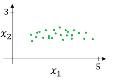
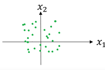
Consider the following example of a training dataset with 2 features, X₁ and X₂. The training dataset can be visualized as the scatterplot shown below:

Normalization is a two-step process.

Step 1 - Subtract the mean

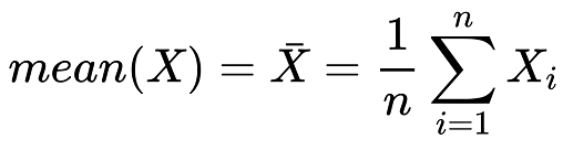
The mean of the dataset is calculated using the formula shown below, and then is subtracted from each individual training example; effectively shifting the dataset so that it has zero mean.

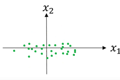
The ranges of both features on their respective axes will be the same, and the result will look like this:

Step 2 - Divide the variance

Notice in the plot above that the feature X₁ has a larger variance (look at the range on the x-axis), than the other feature X₂.
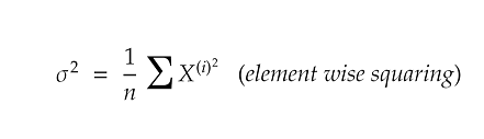
We normalize the variances by applying the formula for variance shown below and then divide each training example with the value of variance thus obtained.

A quick-thinker might have noticed that by dividing each training example with this value, the variance for both X₁ and X₂ will be equal to 1. The scatterplot will now look like the following:

Tip - Use the same values of mean and variance obtained above to normalize your testing dataset too. It is better to scale your testing dataset in the same way you scale your training dataset, so they undergo the same transformation. You will not have to recalculate these values while testing again.

It is also useful to ensure that the input data is in the range of -1 to 1. This avoids issues that arise with floating point number precision. Computers lose accuracy when performing operations on really large or really small numbers (to learn more, check the further reading section at the end of this post).

How significant is Normalization?

Normalization helps significantly effect the performance of your model for the better.

For example, consider a Machine Learning model that uses an algorithm like Gradient Descent to minimize the cost function. For gradient descent essentially finds the minimum of the cost function (often depicted as a contour plot). When the data is normalized, this contour mapping is symmetrical and gradient descent finds it simpler to reach the mean. It converges quicker than when the data is not normalized; it takes more steps to find its way to the minimum.

This is why we desire features to be on a similar scale, and why we go for normalizing inputs. In cases where one is unsure whether the features need to be normalized or not, it is better to go ahead with normalization as this step is simple and doesn't do any harm anyway. An example of how normalization affects model accuracy is given in the further reading section at the end of this post.

Popular Normalization Techniques

The normalization approach shown above is known as the standard scaler approach, where we scaled the inputs to have zero mean and unit variance. Depending upon your problem type, you may opt for a different normalization strategy. When dealing with images, it is common to normalize the image data by 1/255 to ensure pixel values range between 0 and 1. Some of the other popular normalization techniques are:

Batch Normalization

This popular technique was only proposed a few years ago in 2015, and has gone on to become the most commonly used strategy for deep learning models.

Idea:

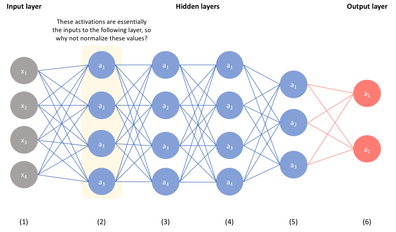
The simple idea is that since the activations of one layer of a neural network are inputs to the following layer, normalizing them too will help the network more effectively learn the parameters in the following layer. Therefore, by normalizing the activations of each layer, one can simplify the overall learning process.

Implementation:

The first couple of steps in implementation are:

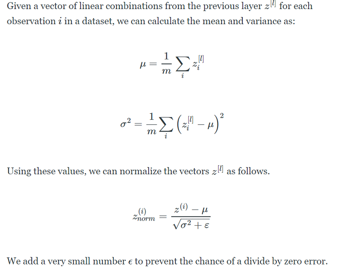
Here z^[l] is the vector output of the previous layer.

An important final step in batch normalization is scaling and shifting the normalized values. For most cases, we do not want out dataset to have zero mean and variance. If we are using activation functions like the sigmoid function then our model performs poorly on such a dataset. So the optimal distribution is given by scaling the normalized values by γ and shifting by β. Note that μ and σ² are calculated per-batch while γ and β are learned parameters used across all batches.

Here is the overall implementation of the Batch Norm algorithm:

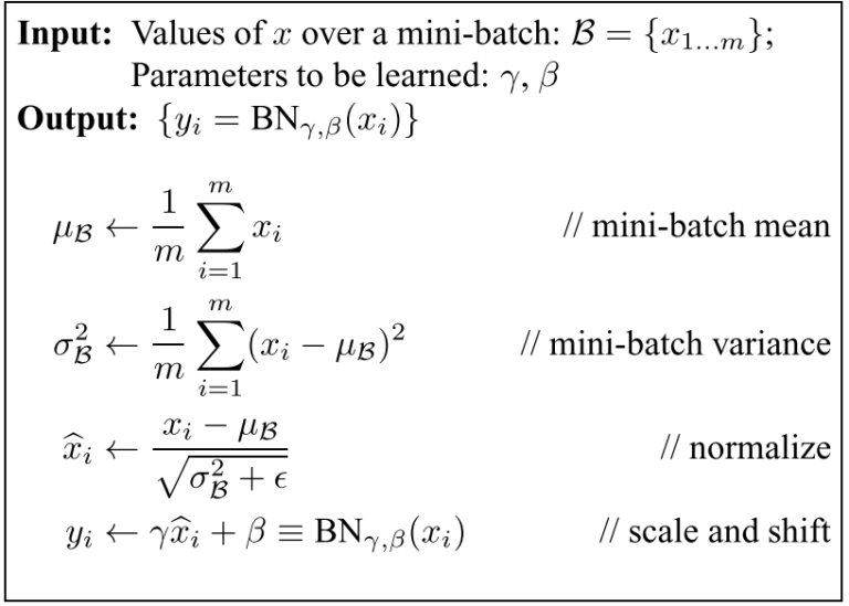
In psuedocode form, this would look like the following -

""" 
Implementation of batch norm
    Inputs:
    - X: Input data of shape (N, C, H, W)
    - gamma: Scale parameter, of shape (C,)
    - beta: Shift parameter, of shape (C,)
    - epsilon: Constant for numeric stability
    Outputs:
    - out: Output data, of shape (N, C, H, W)
"""
    # mini-batch mean
    mean = mean(X)
    # mini-batch variance
    variance = mean((X - mean) ** 2)
    # normalize
    X_hat = (X - mean) * 1.0 / sqrt(variance + epsilon)
    # scale and shift
    out = gamma * X_hat + beta

Issues:

Batch norm has become a widely adopted technique (especially for CNNs). But there are some issues it faces.

• RNNs have recurrent activations, thus each time-step will require a separate batch normalization layer - ultimately making for a complicated model which needs to store the means and variances for each time-step during training.

• Small mini-batches can make estimates noisy. If the batch size is 1, the variance is zero, so we cannot use batch normalization.

This brings us to alternative normalization techniques.

Weight Normalization

This popular technique was only proposed by Open AI, and as the name suggests, instead of normalizing mini-batches, we normalize the weights of the layer.

Idea:

Normalize the weights of the layer instead of normalizing the activations.

Implementation:

The weights are reparameterized using the following formula:

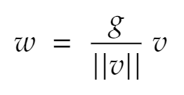
Here, v is a parameter vector and ||v|| denotes the Euclidean norm of v. g is a scalar. This has the effect of fixing the Euclidean norm of the weight vector w: we now have ||w|| = g, independent of the parameters v. This is a similar effect to dividing the inputs by the standard deviation in batch normalization.

The researchers also proposed the idea of combining weight normalization
with a special version of batch normalization, "mean-only batch normalization" - to keep the mean of the activations independent of the parameters v. They subtract out the mean of the mini-batch but do not divide by the standard deviation.

In psuedocode form, this would look like the following -

""" 
Implementation of mean-only batch norm
    Inputs:
    - X: Input data of shape (N, C, H, W)
    - gamma: Scale parameter, of shape (C,)
    - beta: Shift parameter, of shape (C,)
    - v: parameter vector
    - g: scalar value (between 0 and 1), decay constant
    Outputs:
    - out: Output data, of shape (N, C, H, W)
"""
    # mini-batch mean
    mean = mean(X)
    # reparameterize the weights
    w = v/norm(v) * g
    # normalize
    X_hat = X - mean
    # scale and shift
    out = gamma * X_hat + beta

Advantage:

• It can be applied to recurrent models such as LSTMs and also to generative models, unlike simple batch normalization.

Layer Normalization

This technique was proposed by Geoffrey Hinton himself, widely known as the "Godfather of Deep Learning". It is more than a simple reparameterization of the network as in weight normalization.

Idea:

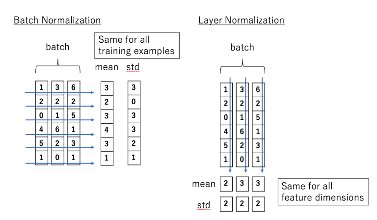
The key idea of layer normalization is that it normalizes the inputs across the features.

Implementation:

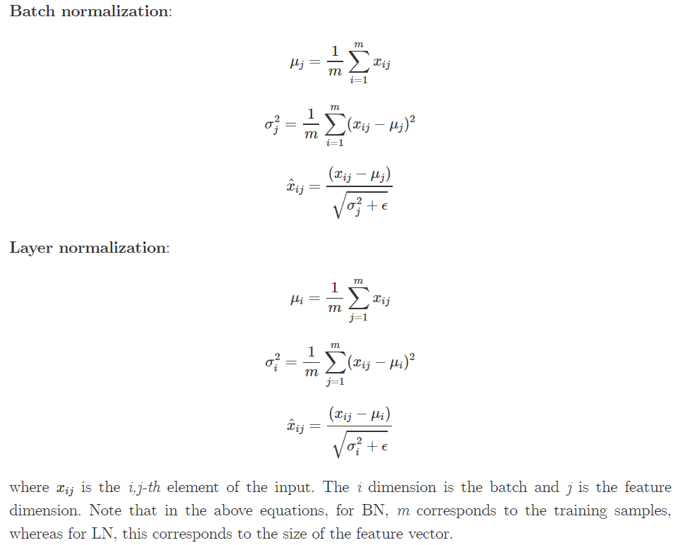
The mean and variance are calculated for each feature and is different for each training example, whereas in batch normalization these statistics re computed across the batch and are the same for each example in the batch. The formulas for both batch norm and layer norm may look similar, but the difference in implementation can best be visualized like this:

Here is a comparison of the formulas involved in batch and layer normalisation. Notice the minute difference in notation.

Advantage:

• Research has shown this technique to be very effective in RNNs.

Learn more:

Test Yourself

With this article at OpenGenus, you must have the complete idea of Normalization and its type. Enjoy.