What's an activation function?
When using machine learning, activation functions are used to transform weighted input from a node to an output value that is passed on to either another layer or can be used as the final output. If we neglected using these, we would simply see linear regression.
A good comparison is thinking about how the brain works. A neuron will get many input signals and its 'activation function' will determine its importance. This activation function would determine whether or not the neuron should be fired.
What is ReLU6?
ReLU6's name is rather descriptive in its definition. This activation function is a modification of ReLU. ReLU is an activator function that is linear in the positive direction and zero in the negative:
f(x) = max(0,x)
ReLU6 uses this same theory but instead limits the positive direction to a maximum size of 6. This is extremely useful when dealing with fixed-point inference. By bounding the upper limit to 6, it allows for more float positions thus being more precise.
f(x) = min(max(0,x),6)
How does ReLU6 differ from other activation functions?
The differences are best shown with code. Note that the code examples are in Python. You will need the modules sklearn, keras, and matplotlib to run these examples if you wish to try them yourself.
Tanh, or hyperbolic tanget, uses the range of -1 and 1 as its activation function. This performs better than the original method of using a sigmoid function when using multiple layers in a neural network. However, as you can see in this code example, as more layers are added, this activation begins to fall apart.
First, we will generate a dataset. In the code example, we are using make_circles to plot random samples and scale them to -1, 1. We then generate test and train values, and define the model. Note that we are using 10 shadow layers here; as you add more shadow layers, you increase the complexity of the problem with each shadow layer. This is known as the vanishing gradient problem.
tanh
from sklearn.datasets import make_circles
from matplotlib import pyplot
from sklearn.preprocessing import MinMaxScaler
from keras.layers import Dense
from keras.models import Sequential
from keras.optimizers import SGD
from keras.initializers import RandomUniform

# Generate dataset
X, y = make_circles(n_samples=600, noise=0.1, random_state=1)
scaler = MinMaxScaler(feature_range=(-1, 1))
X = scaler.fit_transform(X)

n_train = 500
trainX, testX = X[:n_train, :], X[n_train:, :]
trainy, testy = y[:n_train], y[n_train:]

# Define model
init = RandomUniform(minval=0, maxval=1)
model = Sequential()
model.add(Dense(5, input_dim=2, activation='tanh', kernel_initializer=init))
model.add(Dense(5, activation='tanh', kernel_initializer=init))
model.add(Dense(5, activation='tanh', kernel_initializer=init))
model.add(Dense(5, activation='tanh', kernel_initializer=init))
model.add(Dense(5, activation='tanh', kernel_initializer=init))
model.add(Dense(5, activation='tanh', kernel_initializer=init))
model.add(Dense(5, activation='tanh', kernel_initializer=init))
model.add(Dense(5, activation='tanh', kernel_initializer=init))
model.add(Dense(5, activation='tanh', kernel_initializer=init))
model.add(Dense(5, activation='tanh', kernel_initializer=init))
model.add(Dense(5, activation='tanh', kernel_initializer=init))
model.add(Dense(1, activation='sigmoid', kernel_initializer=init))

# Compile the model
opt = SGD(learning_rate=0.01, momentum=0.9)
model.compile(loss='binary_crossentropy', optimizer=opt, metrics=['accuracy'])

# Configure and plot model
history = model.fit(trainX, trainy, validation_data=(
    testX, testy), epochs=500, verbose=0)

_, train_acc = model.evaluate(trainX, trainy, verbose=0)
_, test_acc = model.evaluate(testX, testy, verbose=0)
print('Train: %.3f, Test: %.3f' % (train_acc, test_acc))

pyplot.plot(history.history['accuracy'], label='train')
pyplot.plot(history.history['val_accuracy'], label='test')
pyplot.legend()
pyplot.show()
As shown in the plot, this is not a great solution when using many shadow layers.
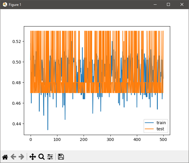
So let's see how this compares to ReLU and ReLU6!
ReLU
This is basically the same exact setup, but this time we change the input and shadow layers to use ReLU as the activation function. ReLU and ReLU6 are far better solutions towards solving the aforementioned vanishing gradient problem.
from sklearn.datasets import make_circles
from matplotlib import pyplot
from sklearn.preprocessing import MinMaxScaler
from keras.layers import Dense
from keras.models import Sequential
from keras.optimizers import SGD
from keras.initializers import RandomUniform

# Generate dataset
X, y = make_circles(n_samples=600, noise=0.1, random_state=1)
scaler = MinMaxScaler(feature_range=(-1, 1))
X = scaler.fit_transform(X)

n_train = 500
trainX, testX = X[:n_train, :], X[n_train:, :]
trainy, testy = y[:n_train], y[n_train:]

# Define model
init = RandomUniform(minval=0, maxval=1)
model = Sequential()
model.add(Dense(5, input_dim=2, activation='relu',
          kernel_initializer='he_uniform'))
model.add(Dense(5, activation='relu', kernel_initializer='he_uniform'))
model.add(Dense(5, activation='relu', kernel_initializer='he_uniform'))
model.add(Dense(5, activation='relu', kernel_initializer='he_uniform'))
model.add(Dense(5, activation='relu', kernel_initializer='he_uniform'))
model.add(Dense(5, activation='relu', kernel_initializer='he_uniform'))
model.add(Dense(5, activation='relu', kernel_initializer='he_uniform'))
model.add(Dense(5, activation='relu', kernel_initializer='he_uniform'))
model.add(Dense(5, activation='relu', kernel_initializer='he_uniform'))
model.add(Dense(5, activation='relu', kernel_initializer='he_uniform'))
model.add(Dense(5, activation='relu', kernel_initializer='he_uniform'))
model.add(Dense(1, activation='sigmoid'))

opt = SGD(learning_rate=0.01, momentum=0.9)
model.compile(loss='binary_crossentropy', optimizer=opt, metrics=['accuracy'])

# Configure and plot model
history = model.fit(trainX, trainy, validation_data=(
    testX, testy), epochs=500, verbose=0)

_, train_acc = model.evaluate(trainX, trainy, verbose=0)
_, test_acc = model.evaluate(testX, testy, verbose=0)
print('Train: %.3f, Test: %.3f' % (train_acc, test_acc))

pyplot.plot(history.history['accuracy'], label='train')
pyplot.plot(history.history['val_accuracy'], label='test')
pyplot.legend()
pyplot.show()
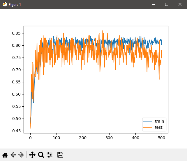
As you can see here, this does a MUCH better job than Tanh using the same dataset.
ReLU6
Finally, we have ReLU6. Again, the only changes we need to make is setting the activation to relu6.
from sklearn.datasets import make_circles
from matplotlib import pyplot
from sklearn.preprocessing import MinMaxScaler
from keras.layers import Dense
from keras.models import Sequential
from keras.optimizers import SGD
from keras.initializers import RandomUniform

# Generate dataset
X, y = make_circles(n_samples=600, noise=0.1, random_state=1)
scaler = MinMaxScaler(feature_range=(-1, 1))
X = scaler.fit_transform(X)

n_train = 500
trainX, testX = X[:n_train, :], X[n_train:, :]
trainy, testy = y[:n_train], y[n_train:]

# Define model
init = RandomUniform(minval=0, maxval=1)
model = Sequential()
model.add(Dense(5, input_dim=2, activation='relu6',
          kernel_initializer='he_uniform'))
model.add(Dense(5, activation='relu6', kernel_initializer='he_uniform'))
model.add(Dense(5, activation='relu6', kernel_initializer='he_uniform'))
model.add(Dense(5, activation='relu6', kernel_initializer='he_uniform'))
model.add(Dense(5, activation='relu6', kernel_initializer='he_uniform'))
model.add(Dense(5, activation='relu6', kernel_initializer='he_uniform'))
model.add(Dense(5, activation='relu6', kernel_initializer='he_uniform'))
model.add(Dense(5, activation='relu6', kernel_initializer='he_uniform'))
model.add(Dense(5, activation='relu6', kernel_initializer='he_uniform'))
model.add(Dense(5, activation='relu6', kernel_initializer='he_uniform'))
model.add(Dense(5, activation='relu6', kernel_initializer='he_uniform'))
model.add(Dense(1, activation='sigmoid'))

opt = SGD(learning_rate=0.01, momentum=0.9)
model.compile(loss='binary_crossentropy', optimizer=opt, metrics=['accuracy'])

# Configure and plot model
history = model.fit(trainX, trainy, validation_data=(
    testX, testy), epochs=500, verbose=0)

_, train_acc = model.evaluate(trainX, trainy, verbose=0)
_, test_acc = model.evaluate(testX, testy, verbose=0)
print('Train: %.3f, Test: %.3f' % (train_acc, test_acc))

pyplot.plot(history.history['accuracy'], label='train')
pyplot.plot(history.history['val_accuracy'], label='test')
pyplot.legend()
pyplot.show()
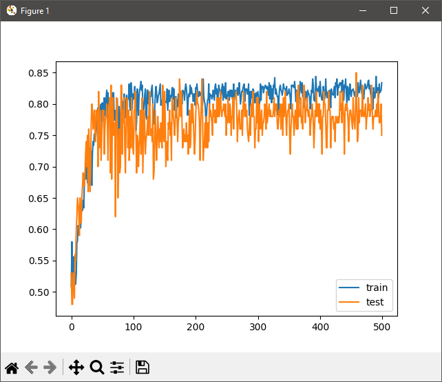
Running this shows the following. Note the differences ReLU6 and ReLU are far less a leap from using tanh, but the key takeaway is there is greater precision with the ReLU6 activation method, thus being a more robust solution.