Ridge Regression

Reading time: 25 minutes | Coding time: 10 minutes

First, we will review the concepts of overfitting and regularization which form the basis of Ridge Regression.

Overfitting

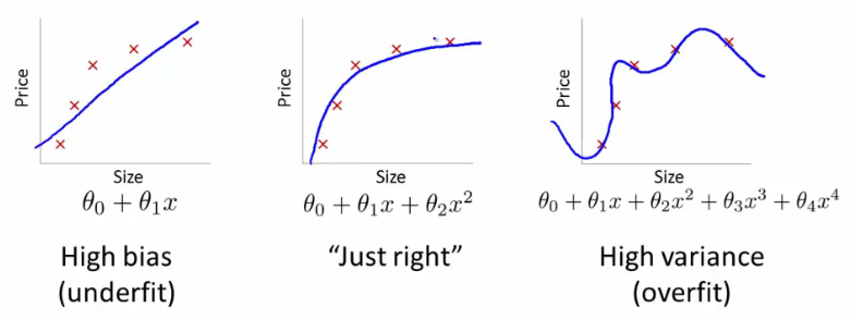
Often in Machine Learning problems, especially with those in which the data set has a large number of features, we can sometimes fit our model too well. This leads to a problem called Overfitting, which basically means that our model has been fitted much better to the training data than needed, and is unable to make accurate prediction on new data. An approach to solve this problem is Regularization.

Regularization

Regularization is the process of adding information in order to solve an ill-posed problem or to prevent overfitting

Basically, we aim to add an extra weight term to our function, in order to add a bit of bias, so that the model 'fits the training data a bit poorly', in order to be much more robust to any new testing data.

There are two types of Regression:

• L1 Regression (Lasso Regression)
• L2 Regression (Ridge Regression)

The key difference between these two is the penalty term that we add:

• In Lasso Regression, we add the absolute value of magnitude of coefficients
• In Ridge Regression, we add the squared magnitude of coefficients

Understanding the Ridge Regression equation

Regression problems involve a Cost function J, which calculates the squared error differences between our predicted values (h(x)) and the actual labels (y) of the target variable, for m number of training examples.

We add a penalty term, in order to make our model more robust and less sensitive to outliers in our dataset.

This is the term given in the second half of the equation. Theta are the weights of our regression model, which we square and calculate the sum of in Ridge Regression.
We multiply that by a coefficient lambda, which is very important in determining the extent of regularization.

Use of L2 regularization in Ridge Regression

Ridge Regression belongs a class of regresion tools that use L2 regularization.

The other type of regularization, L1 regularization, limits the size of the coefficients by adding an L1 penalty equal to the absolute value of the magnitude of coefficients. This sometimes results in the elimination of some coefficients altogether, which can yield sparse models.

L2 regularization adds an L2 penalty, which equals the square of the magnitude of coefficients. All coefficients are shrunk by the same factor (so none are eliminated). Unlike L1 regularization, L2 will not result in sparse models.

Significance of lambda (λ)

Lambda is known as the regularization parameter in Ridge Regression. It can drastically change our model, according to how the value is chosen.

λ = 0: If lambda is 0, we can discard the regularization term entirely, and we get back to our squared error function. This value of lambda is when we don't use regularization at all, and are not trying to solve the problem of overfitting.

0 < λ < ∞: This is when the problem of overfitting is solved. However, the value of λ must be chosen carefully. If it's too less, there will still be overfitting, and if it's too large, we the model can underfit the data.

λ = ∞: If lambda is ∞, the weights of the model, will all become zero, because we have a lot of weightage on the regularization term, i.e on the squares of the weights.

Code

Implementation of Ridge Regression in Sklearn is very simple. Here's a code snippet showing the steps involved:

from sklearn.linear_model import Ridge
import numpy as np
n_samples, n_features = 10, 5
np.random.seed(0)
y = np.random.randn(n_samples)
X = np.random.randn(n_samples, n_features)
clf = Ridge(alpha=1.0)
clf.fit(X, y)

Advantages

• Ridge Regression solves the problem of overfitting, as just regular squared error regression fails to recognize the less important features and uses all of them, leading to overfitting.
• Ridge regression adds a slight bias, to fit the model according to the true values of the data.
• In datasets where we have the number of features (n) larger than the number of training examples (m), ridge regression becomes crucial, as it performs significantly better than regular sum of squares method.
• The ridge estimator is especially good at improving the least-squares estimate when multicollinearity is present.

Drawbacks

• Ridge regression, although improving the test accuracy, uses all the input features in the dataset, unlike step-wise methods that only select a few important features for regression.
• Ridge regression reduces the coefficients theta to very low values if the feature is not important, but it won't completely make them zero, hence still using the feature in our model. Lasso regression overcomes this drawback.