Scaled-YOLOv4 model

In the previous article, we have discussed about YOLOv4's architecture, and how it became a SOTA (state-of-the-art) model for the object detection task offering the best performance in terms of both speed and accuracy. But it could not beat Google's EfficientDet in terms of overall accuracy on the COCO dataset.

So, the authors of YOLOv4 came back and pushed the YOLOv4 model forward by scaling it's design and scale and thus outperforming the benchmarks of EfficientDet. This resulted in Scaled-YOLOv4 model.

Table of contents:

1. The Need for Model Scaling
2. Concept of Model Scaling
3. General Principle
4. Scaling on different devices
5. Scaling Principles for High-End Devices (GPU)
6. Designing Scaled-YOLOv4
7. Results
8. Differences between YOLOv4 and Scaled-YOLOv4

The Need for Model Scaling:

A tremendous amount of progress has been made in the recent years to improve the accuracy of object detectors. The SOTA object detectors improve the accuracy by a great amount but with an increased cost of computation and larger network sizes. This deters their deployment into many real-world applications such as robotics and self-driving cars or embedded systems where size and latency are highly restricted or crucial.

There have been many previous developments aimed to improve the efficiency of the detector architectures, such as one stage and anchor-free detectors or compress existing models. Although these methods were able to achieve better efficiency, but sacrificed on the accuracy part. Main thing to note was that most of these works only focused on a specific or a small range of resource requirements, but the variety of real-world applications, from mobile devices to datacenters, often require a wide variety of resource constraints.

And this raises the need for creating scalable models that can be operated over a wide range of resource constraints.

Concept of Model Scaling:

The traditional way of scaling up a model is to make it more deeper by adding more number of convolutional layers. Later on, width was also increased by increasing the number of filters in each layer, all of this is done with the help of a larger backbone network. To scale up the resolution we will use a larger input image, as this allows detecting smaller objects. A variety of different resolution scaling is performed on the high resolution image and distinct image pyramids (An image pyramid is a collection of images - all arising from a single original image) are obtained. These distinct pyramid combinations are fed to a CNN.

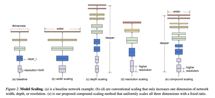
The EfficientDet devised of a compound dimension scaling methodology that improves the efficiency of the model. It scales up all the three parameters - Width, Depth & Resolution.

Scaled-YOLOv4 uses a synergistic compound scaling method.

General Principle:

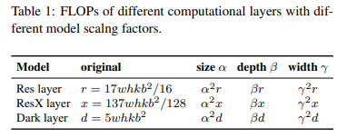
The data below shows the quantitative costs of few of the models when there is a changes in their:

• Image Size
• Number of Layers
• Number of Channels

Let α, β, and γ be their respective scaling factors and they show square, linear and square increase.

We've discussed in the YOLOv4 Architecture Model, about how using Cross Stage Partial strategy reduces the computation costs.

The following are the results obtained after CSP-izing the above models,

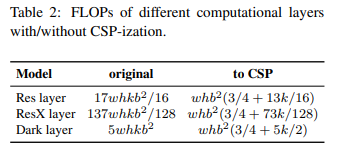
And their improvements are 23.5%, 46.7%, and 50.0%, respectively.

Scaling on different devices:

Scaling Principles for Tiny models on Low-End Devices:

Factors such as memory bandwidth, memory access cost (MACs), and DRAM traffic need to be taken into consideration and the following principles have to be followed:

Order of computation should be less:

It is ideal for tiny models to have a computation order less than O(whkb^2
).
We choose CSP-ized OSANet for the tiny models as it has lower computation complexity.

Minimize/balance size of feature map:

Gradient Truncation between computational block of the CSPOSANet is performed.
b channels of the base layer and the kg channels generated by computational block, and split them into two paths with equal channel numbers i.e (b + kg)/2.

Maintaining same number of channels after convolution:

For evaluating the computation cost of low-end device, we must also consider power consumption, and memory access cost (MAC) is one of the biggest factor affecting power consumption.

Minimize (CIO):

CIO (Convolutional Input/Output) is an indicator that can measure the status of DRAM IO. When kg > b/2, the best CIO is obtained.

Scaling Principles for High-End Devices (GPU):

We are required to find the best combination among the scaling factors when doing the compound scaling. These adjustments are done at the input, backbone, and neck.
The receptive field of the feature vector tells about it's ability to predict the size of an object, and receptive fields are directly related to the stages in the architecture. Thus, higher stages can predict larger objects better.

It is observed that width scaling has no effect on receptive field. It turns out that the compound scaling of input size and stages yields the best results.

Thus, when scaling up compound scaling on input size & stage is performed first, and
then according to real-time requirements, further scaling on depth and width is performed.

Designing Scaled-YOLOv4:

Now we'll talk about the design aspects of the Scaled YOLOv4 for various GPU types.

CSP-ized YOLOv4:

Before we talk about the architecture design, let us look at some of the advantages of using CSP connections:

• Half of the signal going through the main path will generate more semantic information with a large receiving field
• The other half that is being bypassed would preserve more spatial information with a small perceiving field.

Now we talk about the architecture modifications

• This is for General GPUs, YOLOv4 is redesigned to YOLOv4-CSP
• Backbone: The first CSP stage is converted to original Darknet Residual Layer.
• Neck: The PAN architecture is CSP-ized and Mish activation is used to reduce computation by 40%
• SPP: It was originally inserted in the middle position of the neck, the same idea is borrowed and implemented in CSPPAN too.

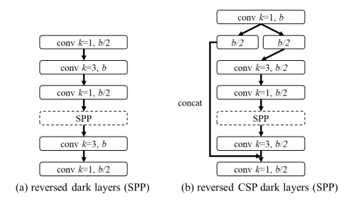
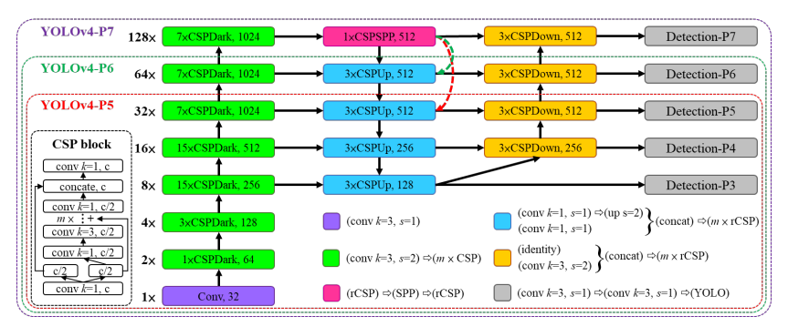
The above is the example of CSP connections in YOLOv4-CSP / P5 / P6 / P7

The entire structure of YOLOv4-CSP can be seen here

YOLOv4-tiny:

• This is designed for the low-end GPU devices.
• This model has been implemented in DarkNet.
• The design follows the principles listed out in the previous section.
• CSPOSANet is used with PCB architecture to form the backbone

YOLOv4-large:

• This is designed for the Cloud GPUs
• Because these are high-performance models, PyTorch was the preferred choice for implementing them.
• The target here is to achieve high accuracy
• YOLOv4-P5 is a fully CSP-ized model, YOLOv4-P6 and YOLOv4-P7 are the scaled models

When we talk about it's implementation it's quite interesting to note that it is written in YOLOv5 PyTorch framework.

Neural Network architecture of Scaled-YOLOv4 (examples of the three networks - P5, P6, P7)

Results:

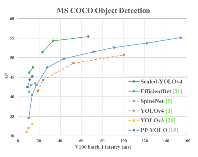
There's no doubt that Scaled-YOLOv4 sets a new standard in object detection.
The main improvement being the ability to efficiently utilize massively parallel devices such as GPUs. This can be confirmed from the results obtained on a GPU V100

YOLOv4-CSP (640x640) — 47.5% AP — 70 FPS — 120 BFlops (60 FMA) Based on BFlops, it should be 933 FPS = (112,000 / 120), but in fact we get 70 FPS, i.e. 7.5% GPU used = (70/933)

EfficientDetD3 (896x896) — 47.5% AP — 36 FPS — 50 BFlops (25 FMA) Based on BFlops, it should be 2240 FPS = (112,000 / 50), but in fact we get 36 FPS, i.e. 1.6% GPU used = (36/2240)

Scaled-YOLOv4 has the same AP50, but a higher AP (predicts better co-ordinates) than the original YOLOv4 with the same resolution and approximately the same speed. The Scaled-YOLOv4 can be scaled up to achieve a higher AP50 and AP at a lower speed.

If we compare the PyTorch & DarkNet implementations of the actual YOLOv4,

YOLOv4(Darknet) — 608x608— 62 FPS — 43.5% AP — 65.7% AP50
YOLOv4(Pytorch) — 608x608 — 62 FPS — 45.5% AP — 64.1% AP50

PyTorch implementation has better co-ordinates prediction but has slightly lower object detection score (AP50)

Then on CSP-izing and using Mish activation and correcting the flaws in PyTorch implementation, we obtain the results as

YOLOv4-CSP(PyTorch) — 608x608–75FPS — 47.5% AP — 66.1% AP50

Differences between YOLOv4 and Scaled-YOLOv4:

As we've seen from the previous article titled "YOLOv4 model architecture", YOLOv4 uses CSP strategy only in it's backbone network. Whereas the YOLOv4-CSP uses a slightly modified CSPDarkNet53 as the backbone and implements CSP in the neck too i.e in the PAN. It employs a compound scaling method with fixed values of the scaling factors - α, β, and γ are fixed so as to scale the network in a constant ratio and in a balanced way. The scaling coefficient is the one parameter that can be varied in-order to scale the network up & accordingly.

With this article at OpenGenus, you must have the complete idea of Scaled YOLOv4 and how it improved over YOLOv4 model.