
Semantic Segmentation is the process of labeling pixels present in an image into a specific class label. It is considered to be a classification process which classifies each pixel. The process of predicting each pixel in the class is known as dense prediction. Image segmentation or semantic segmentation plays a key role in the field of computer vision.

[Semantic Segmentation]
Semantic segmentation is not separating instances of the same class, as we only check for the category of every pixel. To put it in simple words, if there are two or more objects of the same category in our input image , the segmentation process should not distinguish these as separate objects. In order to distinguish separate objects of the same class we use instance segmentation models.
Segmentation models are majorly used to build applications such as:
-
Autonomous Vehicle: Autonomous vehicles are equipped with the perception needed to understand their environment and use semantic segmentation to drive safely.
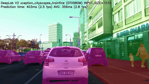
[Autonomous Vehicle in Semantic Segmentation] -
Medical Diagnostics: Semantic segmentation can be used in the field of medical diagnostics as it can help in detecting and identifying several parts of the damaged body and help bring a better cure. It also helps in running faster diagnostic tests.
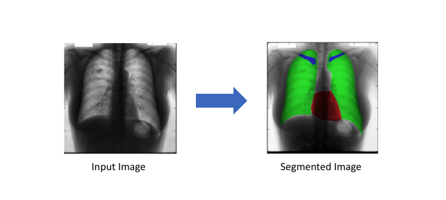
[Medical Diagnostics in Semantic Segmentation]
Examples of semantic segmentation models:
-
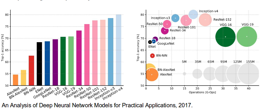
AlexNet: The AlexNet architecture consists of 8 layers in total, out of which there are 5 convolutional layers and 3 fully-connected layers. The Alexnet model was used in the 2012 ImageNet competition.
-
VGG-16: The VGG-16 architecture consists of 16 weighted layers which includes 13 convolutional layers having a filter size of 3 x 3 and 3 fully connected layers. All the convolutional layers present here are divided into groups of 5 and each group is followed by a max pooling layer. This model achieves an accuracy of 92.7%.
-
GoogLeNet: The GoogLenet consists of 9 inception models which are stacked linearly. It has 22 layers or 27 including the pooling layers.It uses global average pooling at the end of the last inception model. Google's network won the 2014 ImageNet competition with an accuracy of 93.3%.
[Architectures used in Semantic Segmentation]
General Structure of Semantic Segmentation model:
[Encoder-Decoder Overview]
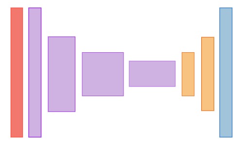
The architecture of a semantic segmentation model 1st goes through a bunch of downsampling layers which are used to decrease the dimensionality of the spatial dimensions. This is then followed by upsampling layers which are used to increase the dimensionality in the spatial dimensions. The output layer however will be the same size as the input layer.
To elaborate the process:
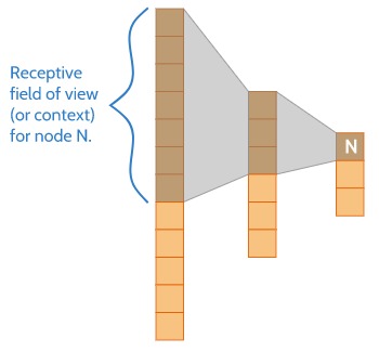
Step 1: The downsampling process involves the model obtaining information about the bigger regions. As the model obtains details about the image it also gets a better understanding of the image. But during this process it also loses spatial information such as the location of the object in the image.
[convolutional-expansion]
Step 2: During the segmentation we tend to keep both forms of information which include the finer details such as the location of the object in the image along with its capability to recognize different objects. This is the reason why a segmentation model passes on the information from the previous layer to the upsampling layer.
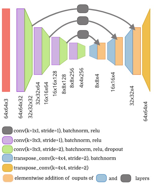
[model-architecture]
Step 3: The information which is further passed along to the other layers and later combined as different for different architectures. Architectures such as the Segnet keep only the indices of the elements which are usually preserved using the maxpool operation. The reverse max-pooling layer is used along with the indices. Other architectures have the entire output being passed along.
Step 4: The purpose of upsampling is to ensure that we end up with the same spatial dimension of the input image. However the number of channels of the output layer will be different from the input image.
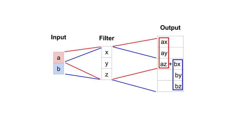
Step 5: The process of upsampling is also different for different architectures. For instance many architectures also use the process of transpose convolution also called de-convolution. The process of deconvolution involves taking a single value from a low resolution feature map and multiplying all of the weights and projecting the weighted values onto the feature map. In simpler words it makes a bigger feature map instead of a smaller feature map.
[Transposed-Operation]
Another technique for upsampling is max un-pooling operation. This technique captures the example specific structures by tracing the original locations with the help of strong activation. This results in effectively reconstructing the detailed structure.
Now that we have the general structure of the semantic segmentation, we would now understand how it takes the input and produeces an output.
Inputs, Labels and the Outputs of a Segmentation model:
Inputs:
The input to the segmentation task will be images of regular type. The images could be grayscale or coloured.
Labels:
The labels can differ for different datasets which we use. Since we have class labels for each pixel of the input image. Due to this type the data gets packaged as an array representing a batch of images.
-
The class label can be packaged as grayscale images where the pixel intensity represents a class id of the image. This kind of labelling allows for a small file size for distribution and does not take much preprocessing to work.
-
If the image is an RGB image then the data which is stored as RGB images will have different classes of RGB colors representing it. This method allows us to visualize the data since we can view them using any library. This step does not need any extra preprocessing for the representation of the labels.
-
Another type of labeling is to use one hot encoding to represent a pixel with a value of 1 for the class it represents and 0 for the classes it does not represent.
Outputs:
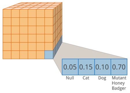
The output which is provided by the semantic segmentation is a tensor. This tensor usually consists of [n_samples, height, width, n_classes]. The output height and width usually has the same size as the original input image. After passing the labels through the softmax function, the final axis consists of the predicted probability distribution of each class for a single pixel.
[Segmentation and Classification]
Now that we understand how the model takes in the input and produeces an output, we now proceed to understand the working of a semantic segmentation model known as "Unet".
Unet:
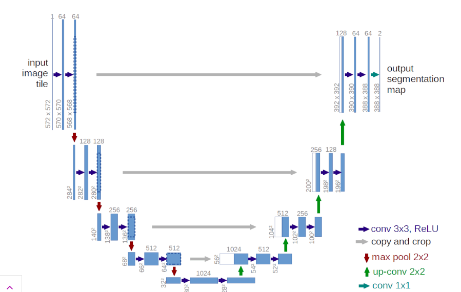
[Unet - Architecture]
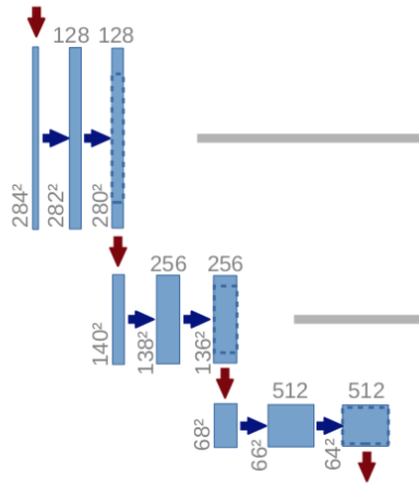
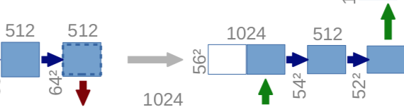
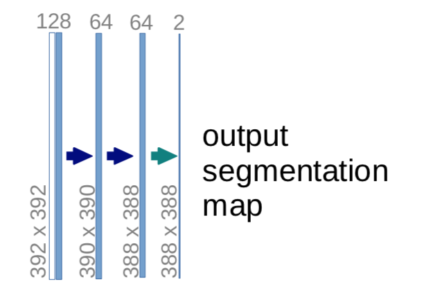
The Unet was originally developed by Olaf Ronneberger et al which was used for Bio Medical Image Segmentation. The U-net architecture consists of two main parts or paths: (i)the encoder (ii)the decoder. The first path is known as the contraction path which is often used to obtain the context in the image. The encoder consists of a stack of convolutional layers along with max-pooling layers. The decoder or the second path is also known as the symmetric expanding path which is used for transposed convolutions and to use precise localization. The Unet is thus a fully connected convolutional layer as it does not contain any dense layer and has only convolutional layers.
The ability of the Unet to precisely localize the borders present in the image is due to the fact that it does classification on every pixel as the input and the output have the same size.
Down sampling/ Contraction/ Encoder Path:
- This path consists of 4 blocks and each block consists of:
- Two convolutional layers of size 3 x 3 along with the ReLU activation function and also utilizes the batch normalization method.
- This layer also has a 2 x 2 max pooling layer.
Up sampling/ Decoder Path:
- This extension path consists of 4 blocks and each block consists of:
- A single Deconvolutional layer with a stride of 2.
- Concatenation of the feature map which was obtained from the encoder path. We now use skip-connections in the decoder path in order to concatenate the output from the previous layers of the encoder.
- At the end, it consists of two 3 x 3 convolutional layers accompanied by a ReLU activation function and batch normalization.
Implementation (Using Keras and Python):
Before we understand the code present below, you need to be aware of the basics of python, numpy, matplotlib along with the fundamentals of Keras.
1. We first start with the necessary imports:
import os
import sys
import random
import warnings

import numpy as np
import pandas as pd

import matplotlib.pyplot as plt

from tqdm import tqdm
from itertools import chain
from skimage.io import imread, imshow, imread_collection, concatenate_images
from skimage.transform import resize
from skimage.morphology import label

from keras.models import Model, load_model
from keras.layers import Input
from keras.layers.core import Dropout, Lambda
from keras.layers.convolutional import Conv2D, Conv2DTranspose
from keras.layers.pooling import MaxPooling2D
from keras.layers.merge import concatenate
from keras.callbacks import EarlyStopping, ModelCheckpoint
from keras import backend as K

import tensorflow as tf
2. After this we set the necessary constants which help in regularizing the input and define the train and test paths:
# Set some parameters
BATCH_SIZE = 10
IMG_WIDTH = 128
IMG_HEIGHT = 128
IMG_CHANNELS = 3
TRAIN_PATH = 'input/stage1_train/'
TEST_PATH = 'input/stage1_test/'

seed = 42
3.The next would be to define the training and testing id inorder to refer them during the training process, we do that using the os.walk:
train_ids = next(os.walk(TRAIN_PATH))[1]
test_ids = next(os.walk(TEST_PATH))[1]
4.Inorder to reduce the computational complexity in the data we use the following code:
X_train = np.zeros((len(train_ids), IMG_HEIGHT, IMG_WIDTH, IMG_CHANNELS), dtype=np.uint8)
Y_train = np.zeros((len(train_ids), IMG_HEIGHT, IMG_WIDTH, 1), dtype=np.bool)

print('Obtaining and training the images ')
sys.stdout.flush()
for n, id_ in tqdm(enumerate(train_ids), total=len(train_ids)):
    path = TRAIN_PATH + id_
    img = imread(path + '/images/' + id_ + '.png')[:,:,:IMG_CHANNELS]
    img = resize(img, (IMG_HEIGHT, IMG_WIDTH), mode='constant', preserve_range=True)
    X_train[n] = img
    mask = np.zeros((IMG_HEIGHT, IMG_WIDTH, 1), dtype=np.bool)
    for mask_file in next(os.walk(path + '/masks/'))[2]:
        mask_ = imread(path + '/masks/' + mask_file)
        mask_ = np.expand_dims(resize(mask_, (IMG_HEIGHT, IMG_WIDTH), mode='constant',
                                      preserve_range=True), axis=-1)
        mask = np.maximum(mask, mask_)
    Y_train[n] = mask

# Get and resize test images
X_test = np.zeros((len(test_ids), IMG_HEIGHT, IMG_WIDTH, IMG_CHANNELS), dtype=np.uint8)
sizes_test = [ ]
print('obtaining and reshaping the test images ... ')
sys.stdout.flush()
for n, id_ in tqdm(enumerate(test_ids), total=len(test_ids)):
    path = TEST_PATH + id_
    img = imread(path + '/images/' + id_ + '.png')[:,:,:IMG_CHANNELS]
    sizes_test.append([img.shape[0], img.shape[1]])
    img = resize(img, (IMG_HEIGHT, IMG_WIDTH), mode='constant', preserve_range=True)
    X_test[n] = img
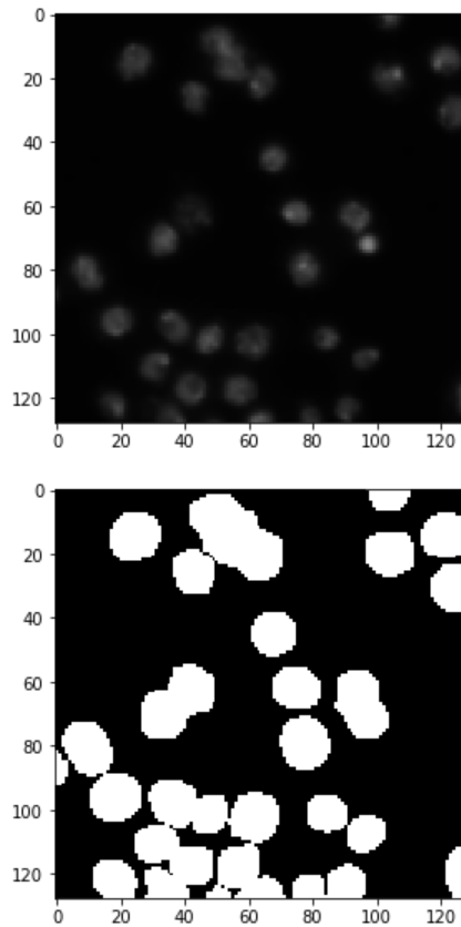
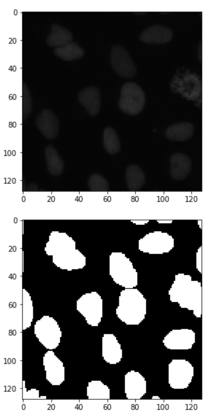
5.The next step is to display the microscopic images in the data using the matplotlib function , this also ensures if the training data is correctly assigned:
ix = random.randint(0, len(train_ids))
imshow(X_train[ix])
plt.show()
imshow(np.squeeze(Y_train[ix]))
plt.show()
The output image of the training data looks as follows:
6. After this we use the mean IOU loss which is commonly used in semantic segmentation as a metric to calculate the Intersection-Over-Union loss and then compute the average over all the classes:
def mean_iou(y_true, y_pred):
    prec = [ ]
    for t in np.arange(0.5, 1.0, 0.05):
        y_pred_ = tf.to_int32(y_pred > t)
        score, up_opt = tf.metrics.mean_iou(y_true, y_pred_, 2)
        K.get_session().run(tf.local_variables_initializer())
        with tf.control_dependencies([up_opt]):
            score = tf.identity(score)
        prec.append(score)
    return K.mean(K.stack(prec), axis=0)
7.The U-net architecture:
inputs = tf.keras.layers.Input((IMG_HEIGHT, IMG_WIDTH, IMG_CHANNELS))
s = tf.keras.layers.Lambda(lambda x: x / 255)(inputs)

c1 = tf.keras.layers.Conv2D(16, (3, 3), activation=tf.keras.activations.elu, kernel_initializer='he_normal',
                            padding='same')(s)
c1 = tf.keras.layers.Dropout(0.1)(c1)
c1 = tf.keras.layers.Conv2D(16, (3, 3), activation=tf.keras.activations.elu, kernel_initializer='he_normal',
                            padding='same')(c1)
p1 = tf.keras.layers.MaxPooling2D((2, 2))(c1)

c2 = tf.keras.layers.Conv2D(32, (3, 3), activation=tf.keras.activations.elu, kernel_initializer='he_normal',
                            padding='same')(p1)
c2 = tf.keras.layers.Dropout(0.1)(c2)
c2 = tf.keras.layers.Conv2D(32, (3, 3), activation=tf.keras.activations.elu, kernel_initializer='he_normal',
                            padding='same')(c2)
p2 = tf.keras.layers.MaxPooling2D((2, 2))(c2)

c3 = tf.keras.layers.Conv2D(64, (3, 3), activation=tf.keras.activations.elu, kernel_initializer='he_normal',
                            padding='same')(p2)
c3 = tf.keras.layers.Dropout(0.2)(c3)
c3 = tf.keras.layers.Conv2D(64, (3, 3), activation=tf.keras.activations.elu, kernel_initializer='he_normal',
                            padding='same')(c3)
p3 = tf.keras.layers.MaxPooling2D((2, 2))(c3)

c4 = tf.keras.layers.Conv2D(128, (3, 3), activation=tf.keras.activations.elu, kernel_initializer='he_normal',
                            padding='same')(p3)
c4 = tf.keras.layers.Dropout(0.2)(c4)
c4 = tf.keras.layers.Conv2D(128, (3, 3), activation=tf.keras.activations.elu, kernel_initializer='he_normal',
                            padding='same')(c4)
p4 = tf.keras.layers.MaxPooling2D(pool_size=(2, 2))(c4)

c5 = tf.keras.layers.Conv2D(256, (3, 3), activation=tf.keras.activations.elu, kernel_initializer='he_normal',
                            padding='same')(p4)
c5 = tf.keras.layers.Dropout(0.3)(c5)
c5 = tf.keras.layers.Conv2D(256, (3, 3), activation=tf.keras.activations.elu, kernel_initializer='he_normal',
                            padding='same')(c5)

u6 = tf.keras.layers.Conv2DTranspose(128, (2, 2), strides=(2, 2), padding='same')(c5)
u6 = tf.keras.layers.concatenate([u6, c4])
c6 = tf.keras.layers.Conv2D(128, (3, 3), activation=tf.keras.activations.elu, kernel_initializer='he_normal',
                            padding='same')(u6)
c6 = tf.keras.layers.Dropout(0.2)(c6)
c6 = tf.keras.layers.Conv2D(128, (3, 3), activation=tf.keras.activations.elu, kernel_initializer='he_normal',
                            padding='same')(c6)

u7 = tf.keras.layers.Conv2DTranspose(64, (2, 2), strides=(2, 2), padding='same')(c6)
u7 = tf.keras.layers.concatenate([u7, c3])
c7 = tf.keras.layers.Conv2D(64, (3, 3), activation=tf.keras.activations.elu, kernel_initializer='he_normal',
                            padding='same')(u7)
c7 = tf.keras.layers.Dropout(0.2)(c7)
c7 = tf.keras.layers.Conv2D(64, (3, 3), activation=tf.keras.activations.elu, kernel_initializer='he_normal',
                            padding='same')(c7)

u8 = tf.keras.layers.Conv2DTranspose(32, (2, 2), strides=(2, 2), padding='same')(c7)
u8 = tf.keras.layers.concatenate([u8, c2])
c8 = tf.keras.layers.Conv2D(32, (3, 3), activation=tf.keras.activations.elu, kernel_initializer='he_normal',
                            padding='same')(u8)
c8 = tf.keras.layers.Dropout(0.1)(c8)
c8 = tf.keras.layers.Conv2D(32, (3, 3), activation=tf.keras.activations.elu, kernel_initializer='he_normal',
                            padding='same')(c8)

u9 = tf.keras.layers.Conv2DTranspose(16, (2, 2), strides=(2, 2), padding='same')(c8)
u9 = tf.keras.layers.concatenate([u9, c1], axis=3)
c9 = tf.keras.layers.Conv2D(16, (3, 3), activation=tf.keras.activations.elu, kernel_initializer='he_normal',
                            padding='same')(u9)
c9 = tf.keras.layers.Dropout(0.1)(c9)
c9 = tf.keras.layers.Conv2D(16, (3, 3), activation=tf.keras.activations.elu, kernel_initializer='he_normal',
                            padding='same')(c9)

outputs = tf.keras.layers.Conv2D(1, (1, 1), activation='sigmoid')(c9)

model = tf.keras.Model(inputs=[inputs], outputs=[outputs])
model.compile(optimizer='adam', loss='binary_crossentropy', metrics=['accuracy'])
model.summary()
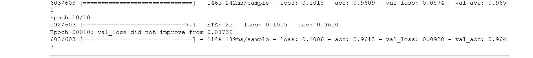
After training the model the 10th epoch shows a result of:
[output-image]
The Downsampling Path:
The downsampling path or the contracting path usually consists of 2 convolutional layers followed by a Max-pooling layers along with a dropout layer(optional)
The first path of the code:
c1 = tf.keras.layers.Conv2D(16, (3, 3), activation=tf.keras.activations.elu, kernel_initializer='he_normal',
                            padding='same')(s)
c1 = tf.keras.layers.Dropout(0.1)(c1)
c1 = tf.keras.layers.Conv2D(16, (3, 3), activation=tf.keras.activations.elu, kernel_initializer='he_normal',
                            padding='same')(c1)
p1 = tf.keras.layers.MaxPooling2D((2, 2))(c1)
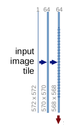
[Downsampling-Path]
This process consists of two convolutional layers which and the number of channels present in each layer will change accordingly. The max-pooling reduces the shape of the image by half which is depicted by the red arrow.
After this the process is repeated twice:
c2 = tf.keras.layers.Conv2D(32, (3, 3), activation=tf.keras.activations.elu, kernel_initializer='he_normal',
                            padding='same')(p1)
c2 = tf.keras.layers.Dropout(0.1)(c2)
c2 = tf.keras.layers.Conv2D(32, (3, 3), activation=tf.keras.activations.elu, kernel_initializer='he_normal',
                            padding='same')(c2)
p2 = tf.keras.layers.MaxPooling2D((2, 2))(c2)

c3 = tf.keras.layers.Conv2D(64, (3, 3), activation=tf.keras.activations.elu, kernel_initializer='he_normal',
                            padding='same')(p2)
c3 = tf.keras.layers.Dropout(0.2)(c3)
c3 = tf.keras.layers.Conv2D(64, (3, 3), activation=tf.keras.activations.elu, kernel_initializer='he_normal',
                            padding='same')(c3)
p3 = tf.keras.layers.MaxPooling2D((2, 2))(c3)

c4 = tf.keras.layers.Conv2D(128, (3, 3), activation=tf.keras.activations.elu, kernel_initializer='he_normal',
                            padding='same')(p3)
c4 = tf.keras.layers.Dropout(0.2)(c4)
c4 = tf.keras.layers.Conv2D(128, (3, 3), activation=tf.keras.activations.elu, kernel_initializer='he_normal',
                            padding='same')(c4)
p4 = tf.keras.layers.MaxPooling2D(pool_size=(2, 2))(c4)
We have the bottom most layer of the U-net architecture which is mostly used to reshape the output from the max-pooling layer. This consists of 2 convolutional layers and no max-pooling layer.
c5 = tf.keras.layers.Conv2D(256, (3, 3), activation=tf.keras.activations.elu, kernel_initializer='he_normal',
                            padding='same')(p4)
c5 = tf.keras.layers.Dropout(0.3)(c5)
c5 = tf.keras.layers.Conv2D(256, (3, 3), activation=tf.keras.activations.elu, kernel_initializer='he_normal',
                            padding='same')(c5)
The UpSampling path:
The upsampling path is used to bring the image back to its original shape using transposed convolution and other up-sampling methods.
u6 = tf.keras.layers.Conv2DTranspose(128, (2, 2), strides=(2, 2), padding='same')(c5)
u6 = tf.keras.layers.concatenate([u6, c4])
c6 = tf.keras.layers.Conv2D(128, (3, 3), activation=tf.keras.activations.elu, kernel_initializer='he_normal',
                            padding='same')(u6)
c6 = tf.keras.layers.Dropout(0.2)(c6)
c6 = tf.keras.layers.Conv2D(128, (3, 3), activation=tf.keras.activations.elu, kernel_initializer='he_normal',
                            padding='same')(c6)
And the process is repeated thrice:
u7 = tf.keras.layers.Conv2DTranspose(64, (2, 2), strides=(2, 2), padding='same')(c6)
u7 = tf.keras.layers.concatenate([u7, c3])
c7 = tf.keras.layers.Conv2D(64, (3, 3), activation=tf.keras.activations.elu, kernel_initializer='he_normal',
                            padding='same')(u7)
c7 = tf.keras.layers.Dropout(0.2)(c7)
c7 = tf.keras.layers.Conv2D(64, (3, 3), activation=tf.keras.activations.elu, kernel_initializer='he_normal',
                            padding='same')(c7)

u8 = tf.keras.layers.Conv2DTranspose(32, (2, 2), strides=(2, 2), padding='same')(c7)
u8 = tf.keras.layers.concatenate([u8, c2])
c8 = tf.keras.layers.Conv2D(32, (3, 3), activation=tf.keras.activations.elu, kernel_initializer='he_normal',
                            padding='same')(u8)
c8 = tf.keras.layers.Dropout(0.1)(c8)
c8 = tf.keras.layers.Conv2D(32, (3, 3), activation=tf.keras.activations.elu, kernel_initializer='he_normal',
                            padding='same')(c8)

u9 = tf.keras.layers.Conv2DTranspose(16, (2, 2), strides=(2, 2), padding='same')(c8)
u9 = tf.keras.layers.concatenate([u9, c1], axis=3)
c9 = tf.keras.layers.Conv2D(16, (3, 3), activation=tf.keras.activations.elu, kernel_initializer='he_normal',
                            padding='same')(u9)
c9 = tf.keras.layers.Dropout(0.1)(c9)
c9 = tf.keras.layers.Conv2D(16, (3, 3), activation=tf.keras.activations.elu, kernel_initializer='he_normal',
                            padding='same')(c9)
The final layer performs a 1 x 1 convolution :
outputs = tf.keras.layers.Conv2D(1, (1, 1), activation='sigmoid')(c9)
After training the model using the we use the training images, we use the test images to validate the data:
ix = random.randint(0, len(test_ids))
imshow(X_train[ix])
plt.show()
imshow(np.squeeze(Y_train[ix]))
plt.show()
This yields results like the image shown below:
Summary:
In summary Unet architecture can be used to perform semantic segmentation and using the API known as keras it can be easily performed. Unet models are great at performing semantic and instance segmentation.
Link to the code: https://github.com/Sandeep-bhuiya/Semantic-Segmentation/blob/master/Semantic Segmentation.ipynb
Link for Extra reading:
https://arxiv.org/abs/1505.04597