In Basics of Time series prediction, We talked about time series where we covered time series data, common patterns in time series data, training ,test and validation sets and statistical forecasting on time series data. We got pretty good results using statistical forecasting on the time series data(mean absolute error = 4.5).

The techniques for Time series prediction are:

• Time Series Forecasting Using Artificial Neural Networks
  • Single Layer Neural Network
  • Recurrent Neural Networks
  • Long Short Term Memory Networks
• Time Series Forecasting Using Stochastic Models
  • Autoregressive moving average model (ARMA)
  • Auto Regressive Integrated Moving Average
  • Seasonal Autoregressive Integrated Moving Average
• Time Series Forecasting Using Support Vector Machines

Time Series Forecasting Using Artificial Neural Networks

Now, let's see how we can improve our results with neural networks. Neural Networks do much of the work for us, and provide us better outputs. They are able to find such relations among the variables which are highly influential and important for predicting the values. We will specifically focus on recurrent neural networks such as Long Short Term Memory(LSTMs) and lambda layers to forecast time series based on given series.

Before starting with RNNs we need to preprocess data in order to use them as variables and labels for our machine learning problem. We can do so with the help of following code:

def windowed_dataset(series, window_size, batch_size, shuffle_buffer):
  dataset = tf.data.Dataset.from_tensor_slices(series)
  dataset = dataset.window(window_size + 1, shift=1, drop_remainder=True)
  dataset = dataset.flat_map(lambda window: window.batch(window_size + 1))
  dataset = dataset.shuffle(shuffle_buffer).map(lambda window: (window[:-1], window[-1]))
  dataset = dataset.batch(batch_size).prefetch(1)
  return dataset

With the above code we will divide our data into:

• Features- number of values in the series
• Labels- label being the next value in the series
• Window size - number of values that will be our feature set, where we're taking a window of the data and training a machine learning model to predict the next value.

from_tensor_slices is used to take values as inputs for value in the dataset. dataset.window defines the window size , here shift attribute in it will truncate the value which are more than our window size. Most of the code we see in this article use numpy arrays so its good to put our data inside numpy list using flat_map function. Next we split the data into features and labels. Shuffle is used to shuffle the values and map split the data into features and labels. Finally we can look at batching the data, and this is done with batch method.

As we have preprocessed our data and our data is ready for a model to be trained on, we will start with single layer neural network.

Single Layer Neural Network

We will use a single layer neural network with a single hidden layer and use it to forecast values. Let's see the code to do so:

dataset = windowed_dataset(x_train, window_size, batch_size, shuffle_buffer_size)
print(dataset)
l0 = tf.keras.layers.Dense(1, input_shape=[window_size])
model = tf.keras.models.Sequential([l0])


model.compile(loss="mse", optimizer=tf.keras.optimizers.SGD(lr=1e-6, momentum=0.9))
model.fit(dataset,epochs=100,verbose=0)

This a single dense layer network with stochastic gradient descent as optimizer in order to modify learning rate and momentum of the model. We measure the loss using mean squared error . Let's look at how good does it forecast on the data

forecast = []

for time in range(len(series) - window_size):
  forecast.append(model.predict(series[time:time + window_size][np.newaxis]))

forecast = forecast[split_time-window_size:]
results = np.array(forecast)[:, 0, 0]


plt.figure(figsize=(10, 6))

plot_series(time_valid, x_valid)
plot_series(time_valid, results)

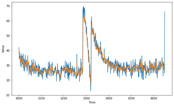
As we can this model forecasts a pretty descent plot. If we calculate the mean squared error , we will get an error of 5.05 which is not that bad but we can do better with the help of recurrent neural networks

Recurrent Neural Networks

The question arises why do recurrent neural networks are preferred for times series data over standard neural network? Well, the reasons for this are :

• The input and outputs can be of different lengths and different examples. So, it's not as if every single example has the same input length / same output length , so it can be a problem in standard neural networks but recurrent neural networks handle it pretty wisely.
• Standard neural networks doesn't share features learned across different positions of time series data.

Recurrent neural networks not only get the data from just previous layer data but also get some information from the previous layers in order to give output. RNNs are able to carry long term dependencies while taking care of short term changes.

Shape of the inputs to the RNN are 3 dimensional . for eg:- if we have a window size of 30 timestamps and we're batching there in sizes of four, the shape will be [4 , 30 , 1] and at each time stamp, the memory cell input will be 4 x 1 matrix.

Let's see a simple recurrent neural network

dataset = windowed_dataset(x_train, window_size, batch_size=128, shuffle_buffer=shuffle_buffer_size)

model = tf.keras.models.Sequential([
  tf.keras.layers.Lambda(lambda x: tf.expand_dims(x, axis=-1),
                      input_shape=[None]),
  tf.keras.layers.SimpleRNN(40, return_sequences=True),
  tf.keras.layers.SimpleRNN(40),
  tf.keras.layers.Dense(1),
  tf.keras.layers.Lambda(lambda x: x * 100.0)
])

optimizer = tf.keras.optimizers.SGD(lr=5e-5, momentum=0.9)
model.compile(loss=tf.keras.losses.Huber(),
              optimizer=optimizer,
              metrics=["mae"])
history = model.fit(dataset,epochs=400)

Now you might be wondering what are lambda layer. So, lambda layer is that layer which allows us to perform arbitrary operations to effectively expand the functionality of tensorflow, keras. This layer will help us deal with dimensionality . Windows_ dataset function which we used, returned 2-D batches of the windows of the data, with the first being the batch_size . But RNN accept 3-D batch-size , number of time stamps and the series of dimensionality. With this we can fix this without modifying our function we used earlier for single layer neural network. Using lambda we extend the layer with 1-D. By setting it to none we're saying that it can take sequence of any length.

You might notice that in the above code we are not using mean squared error as our loss function. Instead of that we are using huber loss function. Huber Loss function is less sensitive to outliers which is useful as this data can get a little bit noisy.

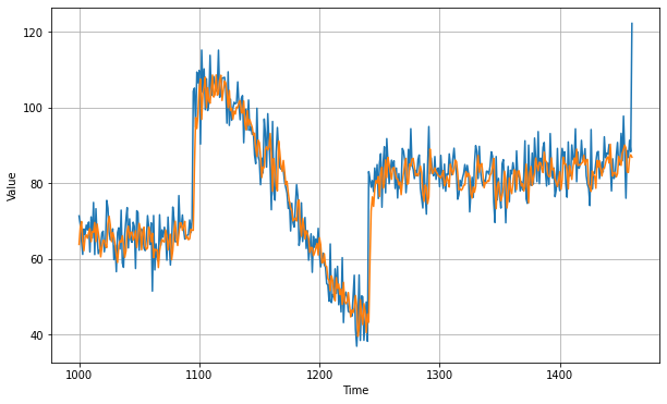
Let's checkout our forecast plot as predicted by our RNN model along with loss function as huber loss function and using stochastic gradient descent as optimizer. We trained our model over 400 epochs and batch size of 128 with learning rate of 5e-5 and momentum = 0.9. We added two simple rnn layers with 40 neurons each which are connected together and then connected to the dense layer with single output. We got the following forecast

As you can see our model gives a good forecast except in the range from 1100 to 1150 due to that sudden heap in the data. This gives us a mean absolute error of 5.99, which is good but not as good as we expected. Let's see how LSTMs can improve this result.

Long Short Term Memory Networks

In Sepp Hochreiter's original paper on the LSTM where he introduces the algorithm and method to the scientific community, he explains that the long term memory refers to the learned weights and the short term memory refers to the gated cell state values that change with each step through time t.

LSTM neyworks maintain a memory cell which is responsible for passing essential information in data seen at earlier steps to the later steps so that the forecast is not fully dependent on the values in the few previous steps and also to avoid problem of vanishing gradient.

dataset = windowed_dataset(x_train, window_size, batch_size, shuffle_buffer_size)

model = tf.keras.models.Sequential([
  tf.keras.layers.Lambda(lambda x: tf.expand_dims(x, axis=-1),
                      input_shape=[None]),
   tf.keras.layers.Bidirectional(tf.keras.layers.LSTM(32, return_sequences=True)),
  tf.keras.layers.Bidirectional(tf.keras.layers.LSTM(32)),
  tf.keras.layers.Dense(1),
  tf.keras.layers.Lambda(lambda x: x * 100.0)
])


model.compile(loss="mse", optimizer=tf.keras.optimizers.SGD(lr=1e-5, momentum=0.9),metrics=["mae"])
history = model.fit(dataset,epochs=200,verbose=1)

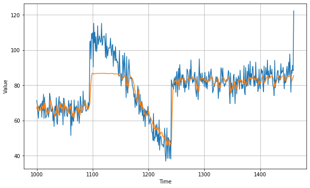
In the above model we are using two bidirectional LSTM layers of 32 neurons each along with the dense layer with 1 output. Bidirectional LSTMs are able to update weights in both direction and can not only pass previous information to forecast future values but can also pass values in the past to forecast the missing time series data values. Here we use mean squared error as loss function and stochastic gradient descent as optimizer.Let's checkout the forecast made by LSTM model.

As you can see our time series is still pretty noisy even though our model gives a better prediction as compared to prediction given by single layer neural network and simple recurrent neural network. If we calculate the mean absolute error we get a value of 3.013. This value is pretty low. This shows that LSTM neural network perform better than simple rnns and single layer neural network. We can further improve our models by tweaking hyperparameters such as learning rate, momentum etc. We can also use other optimizers in place of stochastic gradient descent.

Time Series Forecasting Using Stochastic Models

Autoregressive moving average model (ARMA)

Earlier, in statistical forecasting I described time series in terms of single polynomial moving average(MA). But this model provides description of stationary stochastic time series into two polynomials, one for the autoregression(AR) and another for the moving average(MA). In a time series , the ARMA model is a tool for understanding and, perhaps, predicting future values in this series. The autoregression part regresses the variable on its own lagged (i.e., past) values. The MA part involves modeling the error term as a linear combination of error terms occurring contemporaneously and at various times in the past. The model is usually referred to as the ARMA(p,q) model where p is the order of the AR part and q is the order of the MA part.The notation ARMA(p, q) refers to the model with p autoregressive terms and q moving-average terms. This model contains the AR(p) and MA(q) models,

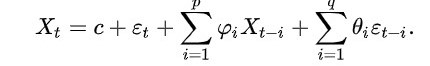
Here the epsilon subscript t is the error terms. The error terms are generally independent identically distributed random variables (i.i.d.) sampled from a normal distribution with zero mean.
ARMA is appropriate when a system is a function of a series of unobserved shocks (the MA or moving average part) as well as its own behavior. For example, stock prices may be shocked by fundamental information as well as exhibiting technical trending and mean-reversion effects due to market participants.

Auto Regressive Integrated Moving Average

Auto Regressive Integrated Moving Average(ARIMA) models explains a given time series data based on its past values, lagged errors and crust and troughs and uses that equation to predict future values.
Any time series which is non-seasonal can be modeled using ARIMA models.An ARIMA model is characterized by 3 terms: p, d, q
where,

p is the order of the AR term

q is the order of the MA term

d is the number of differencing required to make the time series stationary
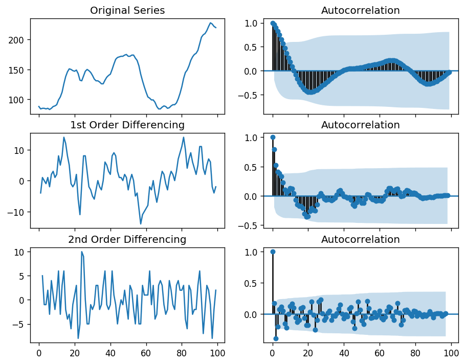
The first step of ARIMA models is to make the time series stationary (we did same when we were doing statistical forecasting), because 'Auto-Regressive' means it is a linear regression model and we know that linear regression models are more accurate when it's predictors are not correlated and is independent of each other. The approach we're gonna use to make it stationary is differencing(we used it back in statistical forecasting).To remove trend and seasonality from the time series with a technique called differencing. So instead of studying the time series itself, we study the difference between the value at time T and value at an earlier period. We can do so using following code:

import numpy as np, pandas as pd
from statsmodels.graphics.tsaplots import plot_acf, plot_pacf
import matplotlib.pyplot as plt
plt.rcParams.update({'figure.figsize':(9,7), 'figure.dpi':120})

# Import data
df = pd.read_csv('https://raw.githubusercontent.com/selva86/datasets/master/wwwusage.csv', names=['value'], header=0)

# Original Series
fig, axes = plt.subplots(3, 2, sharex=True)
axes[0, 0].plot(df.value); axes[0, 0].set_title('Original Series')
plot_acf(df.value, ax=axes[0, 1])

# 1st Differencing
axes[1, 0].plot(df.value.diff()); axes[1, 0].set_title('1st Order Differencing')
plot_acf(df.value.diff().dropna(), ax=axes[1, 1])

# 2nd Differencing
axes[2, 0].plot(df.value.diff().diff()); axes[2, 0].set_title('2nd Order Differencing')
plot_acf(df.value.diff().diff().dropna(), ax=axes[2, 1])

plt.show()

We get the following output after the first order and second order differencing.

Let's build our ARIMA model.

from statsmodels.tsa.arima_model import ARIMA

# 1,1,2 ARIMA Model
model = ARIMA(df.value, order=(1,1,2))
model_fit = model.fit(disp=0)
print(model_fit.summary())

Let’s plot the residuals to ensure there are no patterns (that is, look for constant mean and variance

# Plot residual errors
residuals = pd.DataFrame(model_fit.resid)
fig, ax = plt.subplots(1,2)
residuals.plot(title="Residuals", ax=ax[0])
residuals.plot(kind='kde', title='Density', ax=ax[1])
plt.show()

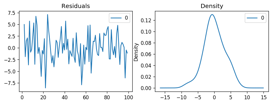
The residual errors seem fine with near zero mean and uniform variance. Let’s plot the actuals against the fitted values using plot_predict().

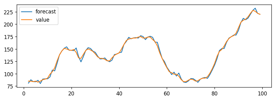
This can make the fitted forecast and actuals look artificially good.

Seasonal Autoregressive Integrated Moving Average

When forecasting periodic data, it is useful to normalize the seasonality out of a dataset. It has become easier to do this with the development of Seasonal Autoregressive Integrated Moving Average, or SARIMA. With the adjustment of hyperparameters, an accurate model can be created. We use SARIMA model because the above ARIMA model is used only for forecasting univariate time series.

A seasonal ARIMA model is formed by including additional seasonal terms in the ARIMA […] The seasonal part of the model consists of terms that are very similar to the non-seasonal components of the model, but they involve backshifts of the seasonal period.
— Page 242, Forecasting: principles and practice, 2013.

Let's build SARIMA model

mod = sm.tsa.statespace.SARIMAX(df.riders, trend='n', order=(0,1,0), seasonal_order=(1,1,1,12))
results = mod.fit()

We can build SARIMA model using above code. SARIMA model can be used to model multivariate time series.

Time Series Forecasting Using Support Vector Machines

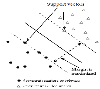
Support Vector Machines(SVMS) are set of supervised learning algorithms used for classification, regression and outliers detection. In a SVM model, given a set of training examples marked to one of the two categories, it assigns the future values to one of the two categories making it a non-probabilistic binary linear classifier(by non probabilistic we mean that it does not give probability as output). SVMs divide the two categories by a canonical hyperplane. This hyperplane is decided by taking a hyperplane which is at equidistant from the closest two points of different categories. SVM kernels are used when suppose your data is not linearly separable by a hyperplane in lower dimensions so we convert the data into higher dimensions using kernels and try finding a hyperplane which can separate the data. The ability of SVM to solve nonlinear regression estimation problems makes SVM successful in time series forecasting.

The huber loss function discussed above can be used as loss function in SVMs for time series prediction as they have low penalizing factor.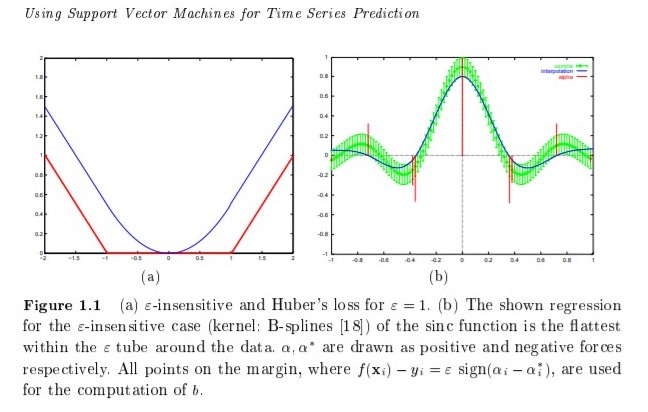

Let's checkout code for the above model:

# prepare sample data in the form of data frame with cols of timesteps (x) and values (y)  
data(AirPassengers) 
monthly_data <- unclass(AirPassengers)
months <- 1:144
DF <- data.frame(months,monthly_data)
colnames(DF)<-c("x","y")

# train an svm model, consider further tuning parameters for lower MSE
svmodel <- svm(y ~ x,data=DF, type="eps-regression",kernel="radial",cost=10000, gamma=10)
#specify timesteps for forecast, eg for all series + 12 months ahead
nd <- 1:156
#compute forecast for all the 156 months 
prognoza <- predict(svmodel, newdata=data.frame(x=nd))

#plot the results
ylim <- c(min(DF$y), max(DF$y))
xlim <- c(min(nd),max(nd))
plot(DF$y, col="blue", ylim=ylim, xlim=xlim, type="l")
par(new=TRUE)
plot(prognoza, col="red", ylim=ylim, xlim=xlim)

We're going to use air passengers dataset that we have seen before. We have monthly data of the air passengers. In the above code we are using radial kernel. We'll compute forecast for all the 156 months. Let's see how well did we compute forecast on it.

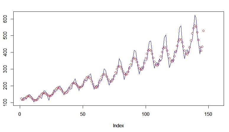
As you can see we did pretty well. We checked out several models for time series prediction in this article at OpenGenus. I have not dwell into exact mathematical equations behind this model. I have given you a glimpse of the maths behind these models. Also, you get better prediction on your data by tuning hyperparameters and preprocessing your data using several techniques.