
Get this book -> Problems on Array: For Interviews and Competitive Programming
In this article, we will explore Gradient Descent Algorithm and it's variants. Gradient Descent is an essential optimization algorithm that helps us finding optimum parameters of our machine learning models.
Table of contents:
In short, there are 3 Types of Gradient Descent:
- Batch Gradient Descent
- Stochastic Gradient Descent
- Mini Batch Gradient Descent
Quick recap on Linear Regression
Although we're not going to use it, you might recall the most famous housing price dataset. You're given features (Age, location, square meters, etc.) about many houses, and their corresponding market prices. What you want to do is to have a linear model that can predict an house price with given features of it. How can we do that? Linear regression is one of the many answers.
Here below we have some x which is our feature and the corresponding y values. In this example, we have simply one feature. What we want to do is to have a system, like in the house example, when a new data point x is given, we can predict what is the corresponding unknown y value.
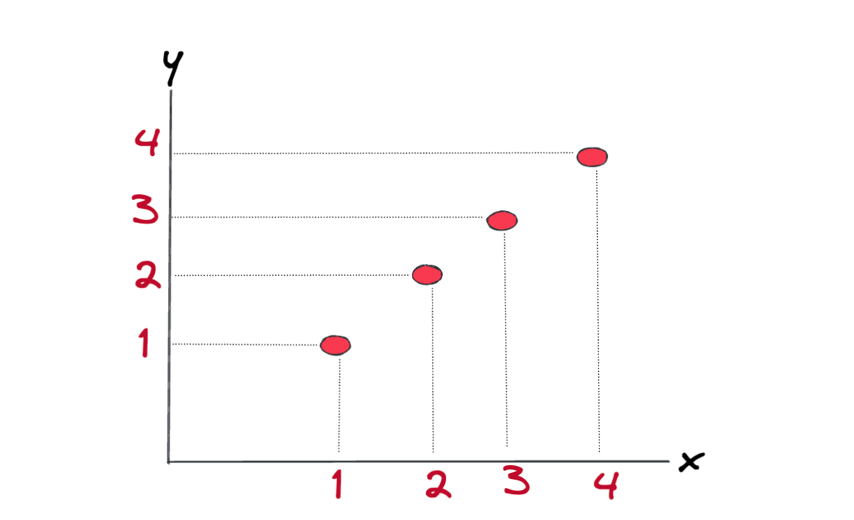
To be able to predict the \(y\) values for the given \(x\), we can use Linear Regression. Here is the formula: ( This is also called as univariate linear regression because we have only one feature.)
$$\hat y = wx + b $$
Parameters
Parameters
- \(\hat y \) is the prediction of the model.
- \(w\) is the weight.
- \(x\) is our feature. Points on the x axis.
- \(b\) is our intercept.
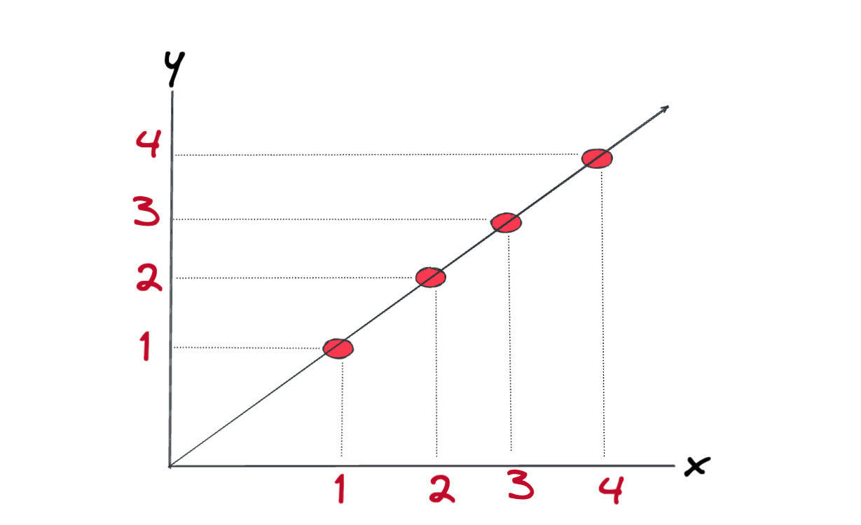
What we want is to have a line which fits our data like the following.
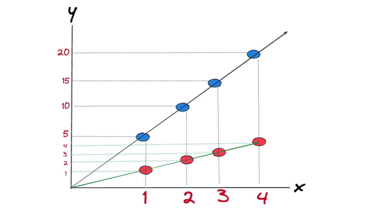
Let's pick \(w=5\) and \(b=0\), for all the data points in our chart, we have:
- \(x_{1}=1\), \(w=5\), \(b=0\), \(\hat y_{1} = 5 * 1 = 5 \),
- \(x_{2}=2\), \(w=5\), \(b=0\), \(\hat y_{2} = 5 * 2 = 10 \),
- \(x_{3}=3\), \(w=5\), \(b=0\), \(\hat y_{3} = 5 * 3 = 15 \),
- \(x_{4}=4\), \(w=5\), \(b=0\), \(\hat y_{4} = 5 * 4 = 20 \)
Blue points are the predicted outcomes for the given points. Clearly, our \(w=5\) is not the best pick. We want to pick such values for \(w\) and \(b\) so that when we plug them into the \(\hat y = wx + b\), they generate the green line. But we need to automate this process, we can't sit and try different values for \(w\) and \(b\), this is where Gradient Descent algorithm becomes handy.
What is Gradient Descent?
Analogy: Suppose that you're lost on a mountain and you want to reach the bottom of valley. You can proceed one step at a time, in the direction of the steepest descent until you reach a place where it's not possible to go further down.Same anology applies while we're trying to find minimum error generating model as well.
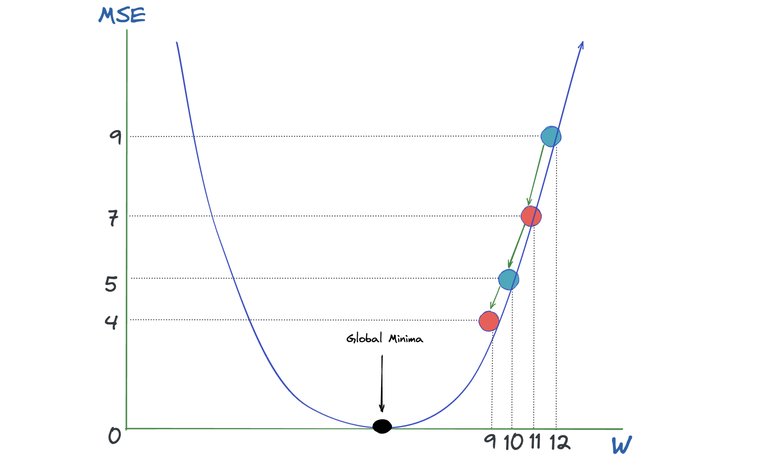
In the below graph, on the Horizontal axis we have our feature \(w\), on the vertical axis we have Mean Squared Errror (MSE). It's a bowl shape which means convex.Therefore we always have a global minima point.This is the point where model generates the smallest possible Mean Squared Errror. Gradient Descent Algorithm is used to find this \(w\) value. It is used all over the place in machine learning, not just for linear regression, but for training for example some of the most advanced neural network models in deep learning.
Note 1: If we have more than one feature, we have local minimas because the function is high dimensional and there are many local minima points.
Note 2: Also, I discard the \(b\) from the equation in the below graph to make it simpler to show.
Here below are the formulas we need to execute Gradient Descent.
$$\ Mean Squared Errror = \frac{1}{2n} * \sum_{i=0}^n {(\hat y_{i} - y_{i})}^2$$ $$ \ w = w - \alpha * \frac{d}{dw}(Mean Squared Errror)$$ $$ \ w = w - \alpha * \frac{1}{n} * \sum_{i=0}^n {(x_{i}*w_{i} - y_{i})}*x_{i}$$
Okay, let's unpack what's going on.
1- We calculate the partial derivative of the MSE with respect to \(w\).
2- We multiply this with \(\alpha\) which is called learning rate. \(\alpha\) allows us to adjust how big our steps going to be. Steps are shown as arrows in the previous graph.
3- We substract this value from our \(w\).
4- We go back to step 2 and repeat it until our MSE doesn't move, which means partial derivative of MSE becomes zero. You can also set up other conditions as well, such as iteration number or threshold on delta between consecutive changes in MSE.
When you also have \(b\) in the equation, we need to compute the new \(w\) as well, which is very similar to how we computed \(w\). Below I inserted the versions of the formulas when we have \(b\) as well.
Note: Remember \(w\) and \(b\) have to be updated at the same time, meaning do not use updated \(w\) in the formula of calculating new \(b\).
Types of Gradient Descent
So far everything seems to be working perfectly, we have an algorithm which finds the optimum values for \(w\) and \(b\). But if you noticed, at every iteration of gradient descent, we're calculating the MSE by iterating through all the data points in our dataset. This gradient descent is called Batch Gradient Descent.
Batch Gradient descent works well when you have small number of data points and small amount of features. Imagine you have hundreds or thousands of features and millions of data points. Well, things get pretty slow at that scenario.
Let's see what are the varients of this algorithm.
-
Stochastic Gradient Descent: In this version, at each iteration, we calculate MSE with only one data point. But since we work with only one training example, when the number of training examples is large, we have to do a lot of iterations in total to be able to find optimal values.
-
Mini Batch gradient descent: In this version at each iteration, we calculate MSE with subset of data points where the number of data points in the subset is a and a < n This version is by far the most effective one. At each iteration, we still capture good amount of training examples, but not all so we can process faster.
Python Code
Here you can find the python code for Batch Gradient Descent, I think it would be a good python exercise for you to change the code and implement Stochastic, and Mini Batch versions :).def gradient_computation(x, y, w, b):
"""
Computes the gradient for linear regression
Argumentss:
x (ndarray (n,)): Data, n examples
y (ndarray (n,)): target values
w,b : model parameters
Returns
dj_dw: The gradient of the cost w.r.t. the parameters w
dj_db: The gradient of the cost w.r.t. the parameter b
"""
# Number of training examples
n = x.shape[0]
dj_dw = 0
dj_db = 0
for i in range(0,n):
f_wb = w * x[i] + b
dj_dw_i = (f_wb - y[i]) * x[i]
dj_db_i = f_wb - y[i]
dj_db += dj_db_i
dj_dw += dj_dw_i
dj_dw = dj_dw / n
dj_db = dj_db / n
return dj_dw, dj_db
def gradient_descent_algorithm(x, y, w_in, b_in, alpha, num_iters, cost_function, gradient_function):
"""
Performs gradient descent to fit w,b. Updates w,b by taking
num_iters gradient steps with learning rate alpha
Args:
x (ndarray (n,)) : Data, n examples
y (ndarray (n,)) : target values
w_in,b_in: initial values of model parameters
alpha: Learning rate
num_iters: number of iterations to run gradient descent
cost_function: function to call to produce cost, cost function's code is not included here.
gradient_function: function to call to produce gradient
Returns:
w: Updated value of parameter after running gradient descent
b: Updated value of parameter after running gradient descent
J_history: History of cost values
p_history: History of parameters [w,b]
"""
# An array to store cost J and w's at each iteration primarily for graphing later
J_history = []
p_history = []
b = b_in
w = w_in
for i in range(num_iters):
# Calculate the gradient and update the parameters using gradient_function
dj_dw, dj_db = gradient_function(x, y, w , b)
# Update Parameters came from gradient_function
b = b - alpha * dj_db
w = w - alpha * dj_dw
# Save cost J at each iteration
if i<100000: # prevent resource exhaustion
J_history.append( cost_function(x, y, w , b))
p_history.append([w,b])
# Print cost every at intervals 10 times or as many iterations if < 10
if i% math.ceil(num_iters/10) == 0:
print(f"Iteration {i:4}: Cost {J_history[-1]:0.2e} ",
f"dj_dw: {dj_dw: 0.3e}, dj_db: {dj_db: 0.3e} ",
f"w: {w: 0.3e}, b:{b: 0.5e}")
return w, b, J_history, p_history #return w and J,w history for graphing