Volumetric Image Segmentation

In this article, we have explored the Machine Learning application: Volumetric Image Segmentation in depth and covered the different ML models used for it like 3D U-Net.

3D data is of two types - surface models and volumetric data. Surface models are seen in the design industry, e.g. polygons or parametric surfaces. Volumetric data is found in the medical market. It means that the inside of the data is also modeled using a discretely sampled 3D set.

Table Of Contents:

1. What Is Volumteric Data?
2. Application(Input & Output)
3. Models for Volumetric Image Segmentation
   • 3D U-Net
   • V-Net
   • UNet++
   • No New-Net
   • VoxResNet
4. Evaluation
5. Conclusion

What Is Volumteric Data?

Volumetric data is a group of 2D image slices, stacked together to form a volume. For example a 3D ultrasound uses sound waves just like a 2D ultrasound, but unlike 2D ultrasound where the waves are transmitted straight through the tissue and organs and back again, the waves are emitted in various angles in a 3D ultrasound which causes a three dimensional view. A volume (3D) image represents a physical quantity as a function of three spatial coordinates.The image is made by a spatial sequence of 2D slices where a slice is represented as a matrix of pixels (X and Y coordinates). The slice number indicates the Z-coordinate. With volumetric imaging a doctor can get access to hundreds of slices of data instead of a couple of images per patient.

Application (Input & Output)

Two strategies are applied to deal with volumetrc inputs. In the first method the 3D volume is cut into 2D slices. These 2D CNNs are trained for segmentation based on intra-slice information. Another method involves extending the network structure to volumetric data by using 3D convolutions and train 3D CNNs for segmentation based on volumetric images. The output is a dense segmentation.

Models for Volumetric Image Segmentation

3D U-Net

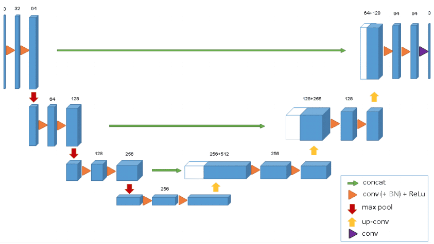
The 3D U-Net was introduced after Unet to process volumes. The model was able to generate dense volumetric segmentation from some 2D annotated slices. Both annotations of new samples could be performed by the network from sparse ones. The average IoU of 0.863 showed that the network was able to find the whole volume from few annotated slices by using a weighted softmax loss function.
One of the cons of the 3D U-Net is that the image size is set to 248 × 244 × 64 and cannot be extended due to memory limitations. Thus the input does not have enough resolution to represent the structure of the entire image. This problem can be solved by dividing the input volume into multiple batches.

V-Net

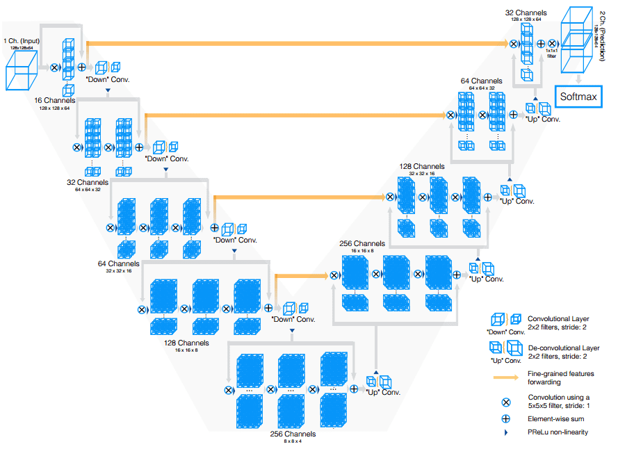
V-Net was derived from U-Net to process 3D MRI volumes. V-Net used 3D convolutions in place of processing the input 3D volumes slice-wise. The modifications in V-Net are:

• They replaced max-pooling operations with strided convolutions. The kernel size is 2 × 2 × 2 with a stride of 2.
• In each stage 3D convolutions with padding are performed using 5 × 5 × 5 kernels.
• In both parts of the network short residual connections are also employed.
• 3D transpose convolutions are utilized in order to extend the dimensions of the inputs. This is followed by one to three conv layers. In every decoder layer we halve the feature maps.

For training only 50 MRI images are used from the PROMISE 2012 challenge dataset. This dataset contains medical data collected from different hospitals, using different equipment and acquisition protocols, to represent the clinical variability.
For testing 30 MRI volumes are processed.

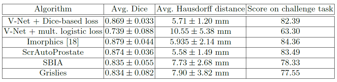
The performance of V-Net using dice loss is better than V-Net with logistic loss.

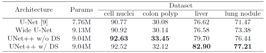
UNet++

High-resolution feature maps directly fast-forwards from the encoder to the decoder network. This leads to the concatenation of semantically dissimilar feature maps. UNet++ tries to improve segmentation accuracy by including Dense block and convolution layers between the encoder and decoder.

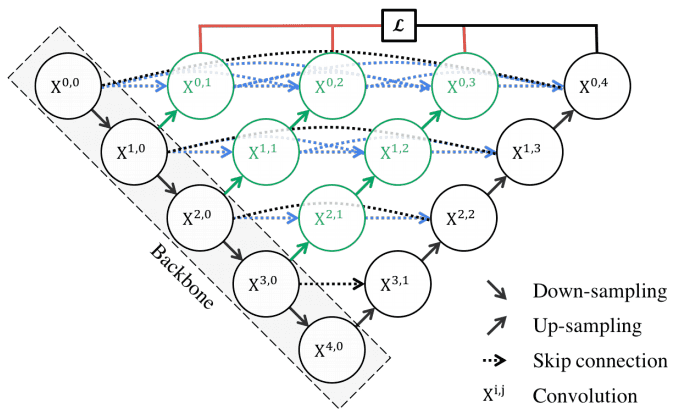
UNet++ have 3 extra features :

• redesigned skip pathways (shown in green)
• dense skip connections (shown in blue)
• deep supervision (shown in red)
  The number of parameters and the time required to train the network is significantly higher.

For evaluation, four medical imaging datasets are used, covering lesions/organs from different medical imaging modalities.

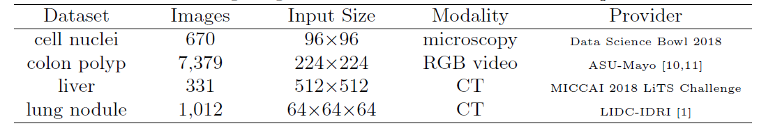
Original U-Net and Wide U-Net(modified U-Net with more kernels such that it has similar number of parameters as the UNet++) are compared.

UNet++ without deep supervision achieves a significant performance gain over both U-Net and wide U-Net, giving average improvement of 2.8 and 3.3 points in IoU.

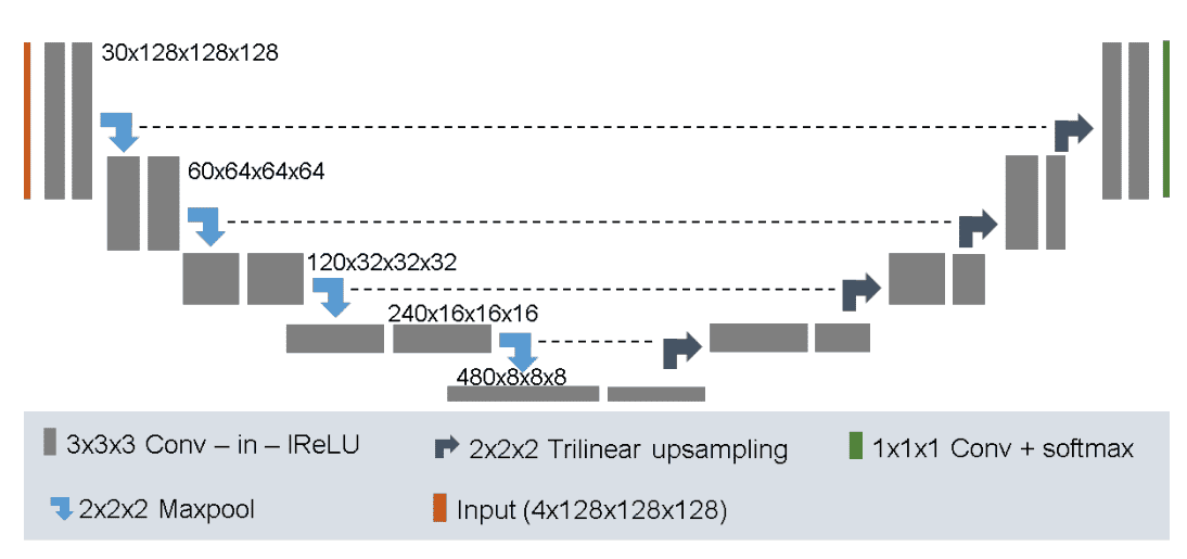
No New-Net

In 3D biomedical image segmentation, dataset propertes like size,voxel spacings, modality etc vary drastically. No New-Net or nnU-Net is the first segmentation method designed to deal with this dataset diversity. nnU-Net uses 128 x 128 x 128 sub-volumes with a batch size of 2. It has 30 channels in the first conv layer and trilinear upsampling in the decoder.

VoxResNet

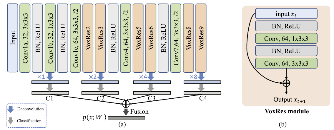
VoxResNet is a deep voxelwise residual network which was extended into a 3D variant for handling volumetric data. A 25 layer model was designed to be applied to brain 3D MRI images. VoxResNet consistes of VoxRes modules where where the input features are added to the tranformed features via a skip connection. 3 convolutional layers are applied with a stride of 2 that ultimately reduced the resolution of input by 8 times. VoxResNet was extended to auto-context VoxResNet or further improving the volumetric segmentation performance. VoxResNet showed Dice coefficients of 0.8696, 0.8061, and 0.8113 for T1, T1-IR, and T2 respectively and 0.885 for the auto-context version.

Evaluation

The task of comparing two segmentations by measuring the distance or similarity between them is called segmentation evaluation. Here one is the segmentation to be evaluated and the other is the corresponding ground truth segmentation. The metrics for volumetric image segmentation can be categorized into the following types:

Spatial overlap based metrics

• The Dice Coefficient (DICE) is the most popular metric in evaluating medial volumetric segmentation. It is defined by:

  DICE = 2TP/2TP +FP +FN
  

• The Jaccard index (JAC) is defined as the intersection between two sets divided by their union, that is

  JAC = TP/TP+FP+FN
  

• Sensitivity and Recall(True Positive Rate (TPR)) measure the portion of positive voxels in the ground truth which are also identified as positive by the segmentation.

  Recall = Sensitivity = TPR =TP/TP +FN
  

• True Negative Rate (TNR) or Specificity, measures the portion of negative voxels (background) in the ground truth segmentation.

  Specificity = TNR = TN/TN +FP
  

• Fβ-Measure (FMS β ) is a tradeoff between precision and recall. Fβ-Measure is given by

  FMSβ = (β^2+1)⋅Precision⋅Recall/β2⋅Precision+Recall
  

When β = 1.0, we get a special case of F1-Measure(FMS). It is also known as harmonic mean and it is given by a

FMS = 2·Precision ·Recall/Precision + Recall

Volume based metrics

• Volumetric similarity (VS) considers the volumes of the segments to indicate similarity.

  VS = 1−(|FN −FP|/2TP +FP +FN)
  

Some other metrics used are Global Consistency Error, Rand Index, Adjusted Rand Index, Probabilistic Distance, Cohens kappa, Area under ROC curve, etc.

Conclusion

In this article at OpenGenus, we saw the basics of volumetric image segmentation and some of the models designed for that purpose and their performances.