
In this article, we will explore different types of cost functions; metrics used to calibrate the model's accuracy iteratively.
Note: You might see in the literature that cost and loss are used in the same context but, there is a distinction. Cost should be used when we're talking about group of objects whereas loss should be used when we're talking about individual instances.
Table of contents:
Why do we need cost functions?
My previous article about Gradient Descent discussed the linear regression model and its parameters. Moreover, I talked about how we use gradient descent to find optimum parameters for b and w so that our model can perform its best.In the gradient descent article, we saw that at every iteration, we have to calculate the Error, and for this, we need a cost function. Ultimately what cost functions do is calculate the individual losses and eventually overall cost. Later this information is fed into gradient descent, and based on the decision of gradient descent, our \(w\)s and \(b\) are updated. This process continues until the overall cost becomes little.
What are different types of cost functions?
The different types of cost functions in Machine Learning are:
- Distance based error
- Mean Squared Error (MSE)
- Mean Absolute Error (MAE)
- Mean Bias Error (MBE)
- Root Mean Squared Error (RMSE)
- Cross Entropy function
We will dive into each cost function.
1) Distance based error
The first cost function is called distance-based error which unites the concept of various cost functions. The model randomizes the w parameters and \(b\), and perform the function \(y = wx + b\) . After the output prediction is \(y'\) is generated, the distance-based error is then calculated as:
$$ Error = \hat y_{i} - y $$
This equation provides the basis for the calculation and use of cost functions for regression problems. But, just calculating the distance-based error function can generate negative errors which is not desirable.
There's a cost function called MBE, where we would like to have negative errors too, I'm going to explain the concept later in this article.
2) Mean Squared Error (MSE)
We already discussed about MSE in gradient descent article. It is one of the most commonly used cost functions in machine-learning, moreover it is simple and straightforward. This function averages the square error values and adds them up. By squaring the error difference, it removes all negative errors.You might also see MSE called as L2 losses in literature. The calculation of it as follows:
$$\frac{1}{N} * \sum_{i=0}^N {(\hat y_{i} - y_{i})}^2$$
1. \(y_{i}\) is the real value.
2. \(\hat y_{i}\) is the predicted value by the model.
3. \(N\) is the total number of observations.
Code:
# This function is called N times, at each time we calculate individual the loss for prediction.
def mse_loss(y_pred, y_true):
    squared_error = (y_pred - y_true) ** 2
    sum_squared_error = np.sum(squared_error)
    loss = sum_squared_error / y_true.size
    return loss
Although MSE is simple and effective it has a major drawback. If a model makes one very poor prediction, the square part of the function will magnify the error. And this results in a huge increase in the overall cost function.
3) Mean Absolute Error (MAE)
MAE is similar in concept to the Mean Squared, but uses the absolute difference of the actual value and the predicted value to eliminate any possibility of negative error. Therefore, we don't need to square which results magnifying the error, and eliminates the drawback of MSE. Moreoever, the MAE score is a linear score, which means that each individual difference is weighted equally in an average.
You might also see MAE called as L1 losses in literature. The formula is given below:
$$\frac{1}{N} * \sum_{i=0}^N |{\hat y_{i} - y_{i}}|$$
1. \(y_{i}\) is the real value
2. \(\hat y_{i}\) is the predicted value by the model.
3. \(N\) is the total number of observations.
Code:
# This function is called N times, at each time we calculate individual the loss for prediction.
def mae_loss(y_pred, y_true):
    abs_error = abs(y_pred - y_true)
    sum_abs_error = np.sum(abs_error)
    loss = sum_abs_error / y_true.size
    return loss
4) Mean Bias Error (MBE)
If the MAE errors signs are not corrected, the average error becomes the MBE. It is intended to measure average model bias in the prediction. MBE can give us some useful information, but you must interpret it cautiously since positive and negative errors will cancel out.$$\frac{1}{N} * \sum_{i=0}^N {\hat y_{i} - y_{i}}$$
1. \(y_{i}\) is the real value
2. \(\hat y_{i}\) is the predicted value by the model.
3. \(N\) is the total number of observations.
5) Root Mean Squared Error (RMSE)
The square root of the MSE is called the Root Mean Squared Error. RMSE can be used when large errors are particularly undesirable. This is how the root mean squared error calculation is done:$${\sqrt {\frac{1}{N} * \sum_{i=0}^N {(\hat y_{i} - y_{i})}^2 }}$$
1. \(y_{i}\) is the real value
2. \(\hat y_{i}\) is the predicted value by the model.
3. \(N\) is the total number of observations.
To diagnose variation in the errors, MAE and RMSE can both be combined. RMSE will always be greater or equal to MAE. If they differ, you should check the magnitude of the difference between them. Below scenarios show us when MAE doesn't change but RMSE increases as the variance associated with the frequency distribution of error magnitudes also increases.
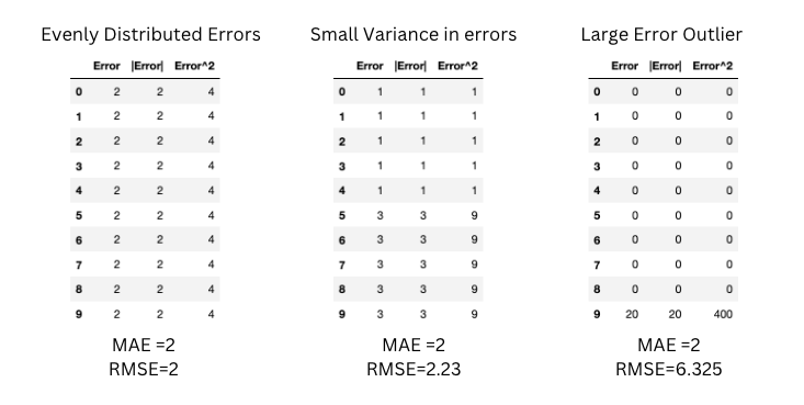
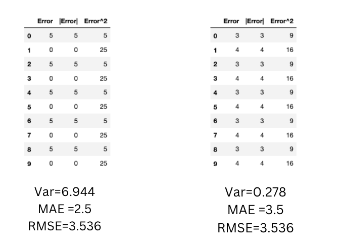
RMSE does not necessarily increase with the variance of the errors. RMSE increases with the variance of the frequency distribution of error magnitudes.
In the below scenarios, the variance of the errors is greater in the first table but the RMSE is the same for both.
Code:
# We can call mse_loss function N times, at each time we calculate individual the loss for prediction.
for i in range(len(y_predict)):
    loss_i = mse_loss (y_pred[i],y_true[i])
    cost += loss_i
RMSE = sqrt(cost)
Okay, so far we discussed the cost functions for regression models,now we will talk about the cost function which is used to asses classification models' performances.
6) Cross Entropy function
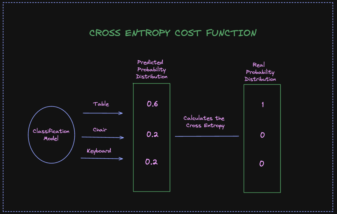
We use Cross Entropy function, also known as log loss function, when we need to measure the performance of our classification models. In this scenario, our model output is a probability value between 0 and 1 . Cross Entropy function measures how far between two probability distributions are. p is an actual probability distribution, and q the predicted probability of the model's output.Cross-entropy measures the deviation between two distributions (Check the image below). A higher deviation between two values means that there is more cross-entropy. Model with a cross entropy 0 is the perfect model.
The calcuation of cross entropy is as follows:
$$ - \sum_{i=0}^N p(x)logq(x) $$
1. \(p(x)\) is the probability distribution of the real values.
2. \(q(x)\) is the probability distribution of the predicted values.
3. \(N\) is the total number of observations.
Code:
def cross_entropy_loss(y_pred ,y_true):
    if y_true == 1:
      return -np.log(y_pred)
    else:
      return -np.log(1 - y_true)
Summary
| Advantages | Disadvantages | ||||||||
|---|---|---|---|---|---|---|---|---|---|
| MSE: Since we square the errors, we penalize huge errors. | MSE: Our advantage of penalizing huge errors can be a disadvantage when we have outliers. | ||||||||
| MSE: We have a gradient descent with only one global minima. | MSE: When a new outlier is added to the data, the model will then produce a different line for the best fit, which could cause results to be skewed. | ||||||||
| MAE: We will weight all errors on the same linear scale because we are taking absolute values. So, unlike MSE, we won’t be placing too much weight upon our outliers. | MAE: Again an advantage can be disadvantage too. The MAE will be less effective if we take into account the outlier predictions made by our model. The outliers' large errors end up being weighted in the exact same way as lower errors. This might mean that our model is great most of the times, but makes a few poor predictions every now-and-then. | ||||||||
| MBE: It can be used to assess the direction of a model. You can check if the bias is positive or negative and correct it. | MBE: It's not a good measurement of magnitude since the errors tend to cancel each other. | ||||||||
| RMSE: It penalizes errors less than MSE because of the square root. | RMSE: It is still sensitive to outliers. | ||||||||
| Cross Entropy: It is very intuitive to work in entropy when dealing with probabilities which makes Cross Entropy a good cost function to use in classification models. | Cross Entropy: Some argue that minimizing the Cross Entropy loss by using a gradient method could lead to a very poor margin if the features of the dataset lie on a low-dimensional subspace.* | ||||||||
Loss functions or cost functions are essential for building and training our models. This article discussed and gave an overview of some of the most important cost functions that are used depending on the type and complexity of the problem.
I hope you find this article useful, until next time take care yourselves!
References:
*https://openreview.net/forum?id=ByfbnsA9Km