The boundary that distinguishes one class from another in a classification issue is known as a decision region in machine learning. It is the region of the input space that translates to a particular output or class.

To put it another way, a decision region is a boundary or surface that divides the input space into regions or subspaces, each of which is associated with a distinct class or category. The specific method utilised for the classification determines whether the decision boundary is linear or non-linear.

The decision border is often shown as a line or curve dividing the two classes in two-dimensional decision regions, but decision regions can also be represented in higher-dimensional space using techniques like scatterplots, heat maps, or contour plots.

Type of Decision Region

Linear decision regions

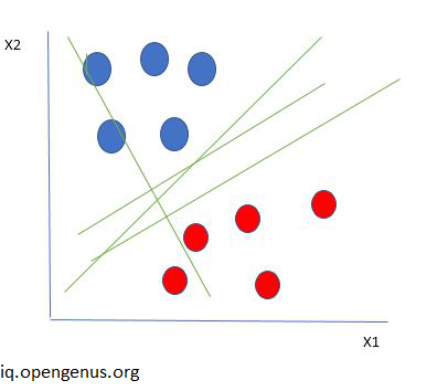
A straight line or a hyperplane that divides the input space into two areas is referred to as a linear decision region because it may be used to represent a decision boundary in the input feature space. The usage of linear decision regions is common in linear classifiers like logistic regression, linear SVM, and perceptrons.
A common formula for a linear decision boundary has the following form:

In other words, w 0 + w 1 * x 1 + w 2 * x 2 +... + w n * x n = 0

where x 1, x 2,..., x n are the characteristics of a data point and w 0, w 1, w 2,..., w n are the weights or coefficients that the linear classifier has learnt.

     |       X
     |      XX
     |     XXXX
     |   XXXX
     |  XX
     | X
     |X
     |
     |             X
     |            XX
     |          XXXX
     |         XXX
     |      XXX
     |    XXX
     |  XX
     |X
     +------------------

Nonlinear decision regions

In other words, the decision boundary is a curved line, a surface, or a complex manifold that divides the input space into several parts. This type of decision boundary is known as a nonlinear decision region. It cannot be represented by a linear equation in the input feature space. Nonlinear decision regions are used by nonlinear classifiers like neural networks, random forests, and decision trees.

Support vector machines (SVMs), a type of kernel algorithm, and non-parametric techniques like decision trees and random forests are among of the most well-liked algorithms for developing nonlinear decision regions.
Using SVMs, the input data is mapped into a higher-dimensional space where a linear decision boundary may be discovered, and this kernel function defines the nonlinear decision boundary. The SVM's decision function is expressed as:

F(x) = sign(sum i, alpha i, y i, K(x i, x) + b)

where K(x i, x) is the kernel function, b is the bias term, and alpha i are the coefficients of the support vectors for each class.

Algorithm on decision regions

Linear Discriminant Analysis (LDA)

The linear decision boundary that maximises the separation between the classes is found via the LDA, a linear classification method. A multivariate Gaussian distribution with a common covariance matrix is used to represent the distribution of each class. Two areas of the input space are divided by the decision boundary, which is a hyperplane.

There are further drawbacks to LDA, such as:

The assumption that the data has a Gaussian distribution may not always be true.
It presupposes that the covariance matrices of the various classes are equal, which could not be the case in some datasets.
Assuming linear separability of the data, which may not be true for all datasets, is what this statement implies.
High-dimensional feature spaces could cause it to struggle.

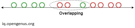
For supervised classification tasks, dimensionality reduction techniques like as linear discriminant analysis, normal discriminant analysis, and discriminant function analysis are frequently utilised. It is used to project the characteristics of a higher-dimension space onto a lower-dimension space to describe distinctions in groups, such as dividing two or more classes.
For instance, we must effectively divide our two classes. Several characteristics are possible for classes. As seen in the following image, using a single characteristic to categorise them may cause some overlapping. Hence, we will continue to add more characteristics to ensure accurate categorization..

Logistic Regression:

A logistic function is used in the linear classification process of logistic regression to predict the likelihood that a data point will belong to a given class. The decision boundary that optimises the likelihood of the practise data is discovered. The decision boundary divides the input space into two areas using a hyperplane.For modelling the likelihood of a binary result based on one or more predictor factors, the logistic regression formula is frequently utilised. Using logistic regression, we can:

p = 1 / (1 + exp(-z))

where:

• p is the predicted probability of the outcome being positive.
• Z is the linear combination of the predictor variables and their associated coefficients, where * p is the predicted probability of a positive outcome, and * * z is the predicted probability of the outcome.
  You may write this as z = 0 + 1x1 + 2x2 +... + pxp.

where:
The intercept, or constant term, is β0 The coefficients, often referred to as weights or parameters, for the predictor variables x1, x2,..., xp are 1, 2,..., p.
Keep in mind that the predictor variables may be continuous, categorical, or a combination of the two.
The logistic function converts a linear combination of predictor variables into a predicted probability value between 0 and 1, which is denoted by the "exp(-z)" term in the formula. This function features an S-shaped curve that gets closer to zero as z app, and it is also known as the sigmoid function.

Support Vector Machines (SVM):

The SVM algorithm, which may be used to classify data in either linear or nonlinear fashion, determines the decision border that optimises the margin between classes. the input data is mapped to a high-dimensional feature space, and the hyperplane that best divides the classes in that space is then found. Two sections of the input space are divided by the decision boundary, which is a hyperplane.

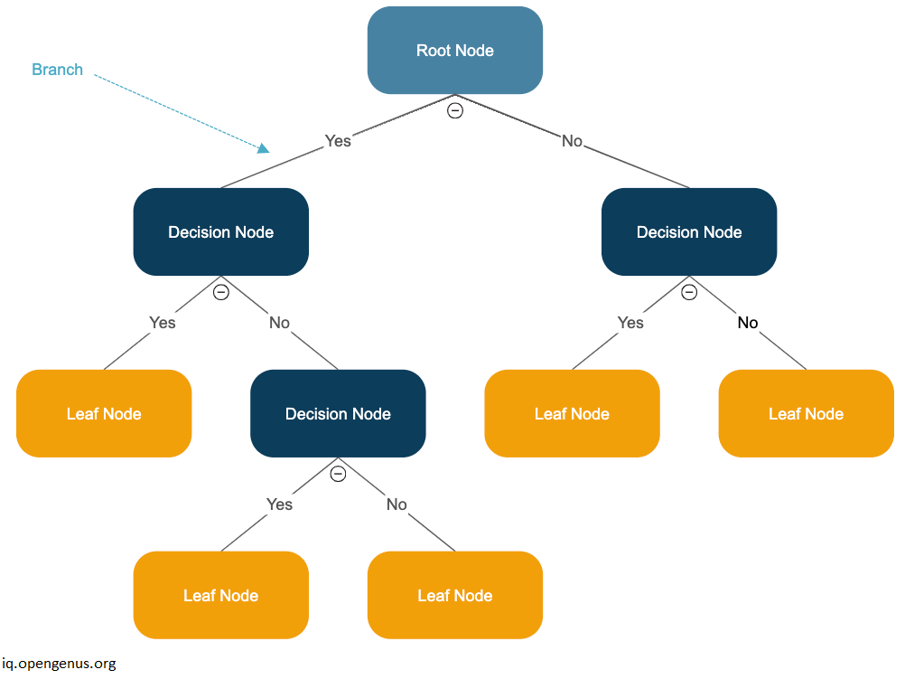
Decision Trees:

A nonlinear classification technique known as a decision tree constructs a model of decisions that resembles a tree depending on the input data. A set of guidelines called the decision boundary is used to decide what class the input characteristics belong to. Depending on the way the tree is structured, the decision boundary may be complicated and nonlinear.

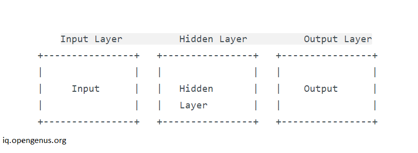
Neural Networks:

An approach for nonlinear classification called a neural network learns a set of weights to translate input information to output classes. They may contain many layers of neurons, enabling them to record nonlinear and complicated decision boundaries. strongly nonlinear and non-convex decision boundary

Decision Regions	Decision Boundary
In a classification issue, the decision boundary is a line dividing the various classes; it is a mathematical function that associates the input data with the appropriate classes. All of the patterns in an useable decision region belong to the same class. A decision region is an area or volume designated by cuts in the pattern space.	The decision region, on the other hand, is the region of the input space that is allocated to a certain class based on the decision boundary and is where the classification algorithm predicts a given class. The area of a problem space known as a decision boundary is where a classifier's output label is unclear. If a hyperplane serves as the decision surface, then the classification issue is linear and the classes are separable along linear paths.

Decision Boundary

from itertools import product

import matplotlib.pyplot as plt

from sklearn import datasets
from sklearn.tree import DecisionTreeClassifier
from sklearn.neighbors import KNeighborsClassifier
from sklearn.svm import SVC
from sklearn.ensemble import VotingClassifier
from sklearn.inspection import DecisionBoundaryDisplay

# Loading some example data
iris = datasets.load_iris()
X = iris.data[:, [0, 2]]
y = iris.target

# Training classifiers
clf1 = DecisionTreeClassifier(max_depth=4)
clf2 = KNeighborsClassifier(n_neighbors=7)
clf3 = SVC(gamma=0.1, kernel="rbf", probability=True)
eclf = VotingClassifier(
    estimators=[("dt", clf1), ("knn", clf2), ("svc", clf3)],
    voting="soft",
    weights=[2, 1, 2],
)

clf1.fit(X, y)
clf2.fit(X, y)
clf3.fit(X, y)
eclf.fit(X, y)

# Plotting decision regions
f, axarr = plt.subplots(2, 2, sharex="col", sharey="row", figsize=(10, 8))
for idx, clf, tt in zip(
    product([0, 1], [0, 1]),
    [clf1, clf2, clf3, eclf],
    ["Decision Tree (depth=4)", "KNN (k=7)", "Kernel SVM", "Soft Voting"],
):
    DecisionBoundaryDisplay.from_estimator(
        clf, X, alpha=0.4, ax=axarr[idx[0], idx[1]], response_method="predict"
    )
    axarr[idx[0], idx[1]].scatter(X[:, 0], X[:, 1], c=y, s=20, edgecolor="k")
    axarr[idx[0], idx[1]].set_title(tt)

plt.show()

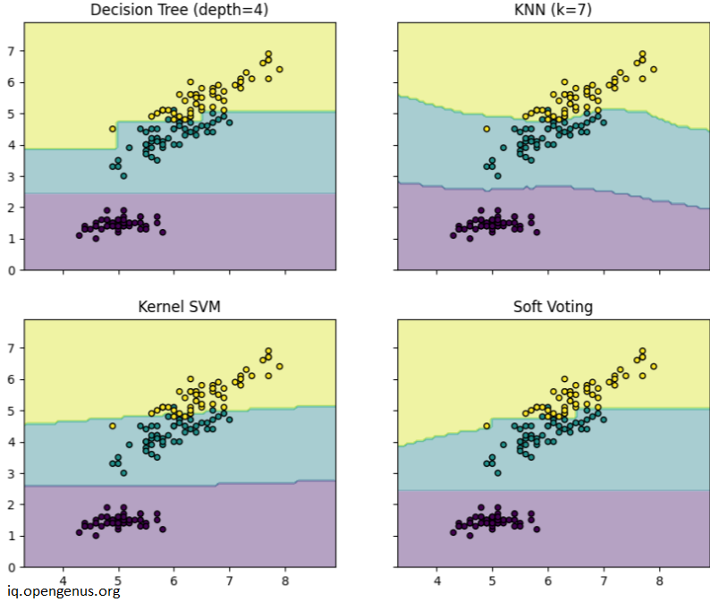
Note the decision boundary and region in the above diagram.

With this article at OpenGenus, you must have the complete idea of Decision Region in Machine Learning.