Reading time: 35 minutes | Coding time: 20 minutes

In this article, we will briefly describe how GANs work, what are some of their use cases, then go on to a modification of GANs, called Deep Convolutional GANs and see how they are implemented using the PyTorch framework.

What if I tell you that you could generate surreal and picturesque paintings on your own, given that you have a large collection of similar paintings at your disposal?

The best part? Nobody would easily find out whether the new painting was made by a human or not!

Or how about the really cool application of generating an image all by your own, described by some text which you provided the model with?

These and many other such awesome use cases are possible thanks to the deep learning architecture known as Generative Adversarial Network (GAN).

Ready? Let's begin!

What are GANs?

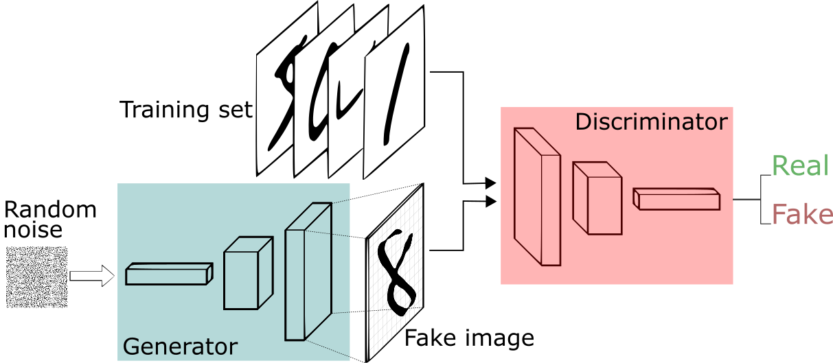
Generative Adversarial Networks are a deep learning architecture based on generative modeling. Their main objective is to generate new data, given lots of similar data as training material.

They achieve this as follows: they have 2 networks - the generator and the discriminator networks.

The purpose of the generator is to generate new samples based on similar samples it is provided with, and the task of the discriminator is to find out whether the image it is assigned is real or produced by the generator network.

The generative model competes with an adversary - a discriminative model that learns to determine whether a sample is from the model distribution (produced by the generator) or the data distribution (original sample).

Some initial noise (usually Gaussian noise) is supplied to the generator network before it begins producing the fake images.

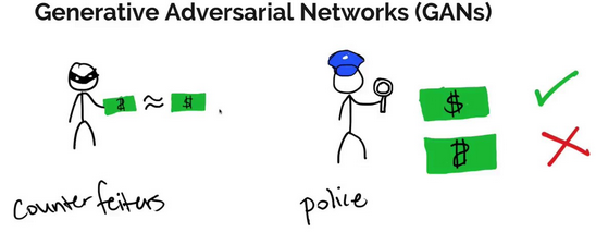
Think of it this way.
The generative model can be thought of as analogous to a team trying to duplicate an original art without getting detected while the discriminative model is analogous to the team trying to detect this.

Competition in this game drives both the teams to improve their methods until the counterfeit articles are indistinguishable from the genuine articles.

GANs represent an unsupervised learning problem (since they aren't provided with training or test labels), where the 2 networks compete, and cooperate with each other at the same time.

It is important that the generator and discriminator don't overpower each other, otherwise the network won't be able to produce fake images of superior quality because the competition will become one-sided.

After all, what's the fun in a game when one team is far stronger than the other, right?

To sum it up, the idea behind GANs is to generate new examples based on training data it is supplied with.

Some applications of GANs

A) Generating examples for Image Datasets

Let's begin with the application GANs were originally created for.

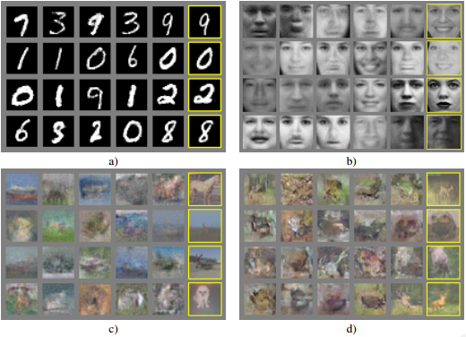
Generating new, credible samples was the application described in the original paper by Goodfellow, et al. (2014) titled "Generative Adversarial Nets" where GANs were used to generate examples for the MNIST handwritten digits dataset, the CIFAR-10 small object photograph dataset, and the Toronto Face Database.

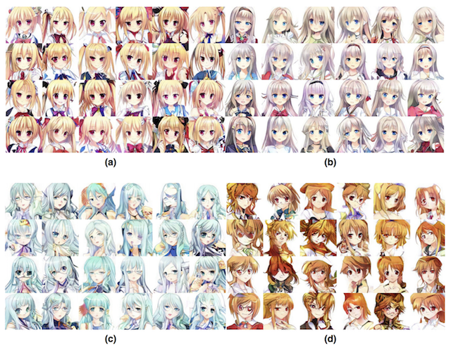
B) Generating Cartoon Characters

Anime lovers, unite!

Jin, et al. (2017) in their paper titled "Towards the Automatic Anime Characters Creation with Generative Adversarial Networks" demonstrate the training and use of a GAN for generating the faces of anime characters.

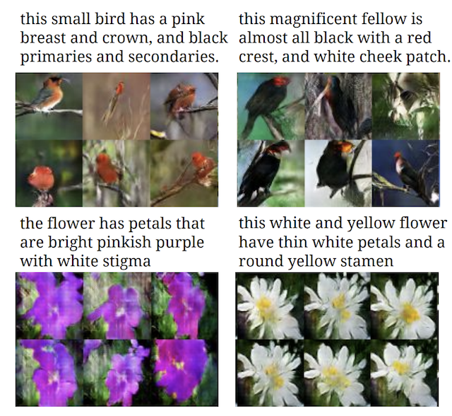
C) Text-to-Image Translation (text2image)

Wouldn't it be amazing if images could be generated on their own with the help of just a few lines of text?

The seemingly possible dream was made into a reality by Zhang, et al. (2016) in their paper "StackGAN: Text to Photo-realistic Image Synthesis with Stacked GANs which illustrate the use of GANs, specifically their StackGAN to generate realistic looking photos from textual descriptions of day-to-day objects like flowers and birds.

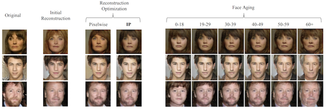
D) Face Aging

You must be savvy with the recent app called "FaceApp", no?

The app takes in an image of a person and generates breathtakingly realistic renditions of the person 3 or 4 decades down the line.

This app is a consequence of the idea of Antipov, et al. (2017) and their paper "Face Aging with Conditional Generative Adversarial Networks" where they use GANs to generate photos of faces with different apparent ages, from younger to older.

So, what are DCGANs?

Using GANs as their inspiration, Radford, et al. (2016) wrote a groundbreaking paper - Unsupervised Representation Learning with Deep Convolutional Generative Adversarial Networks which served as a starting point for using GANs with images.

DCGANs are a class of convolutional GANs, where both the generator and discriminator networks are comprised of convolutional neural networks (CNNs).

This means that DCGANs are perfect for all those applications which require images or videos to be fed to GANs, to generate new and plausible images and videos alike.

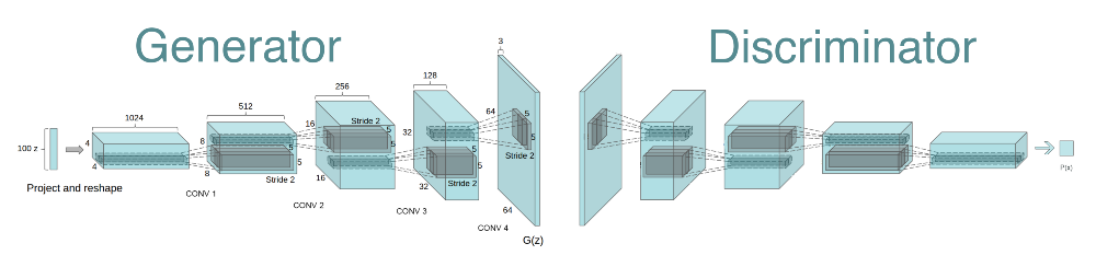
The image shown below is the architecture of the generator network of the DCGAN.

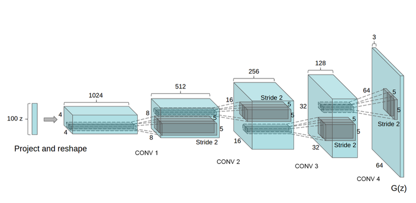
The overall architecture of the model is shown as follows:

Some advantages of DCGANs over GANs include:

1. DCGANs are a more stable architecture for training generative adversarial networks

While GANs gave a test error (on millions of samples) of around 6% on the MNIST dataset, DCGANs only gave an error of 1.48% on 10 million samples.

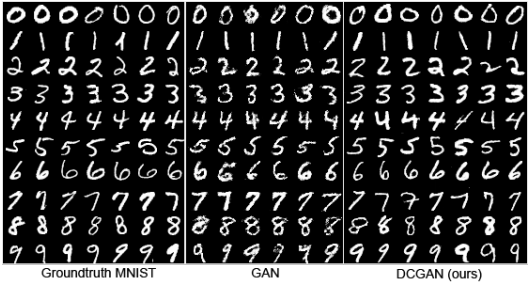
The above image shows the side-by-side (left to right) illustration of the MNIST dataset, generations from a baseline GAN, and generations from a DCGAN.

2. (Technical jargon incoming) They eliminate fully connected layers and replace all the max pooling layers (in the GANs) with convolutional strides.

While the original GAN model trained by Goodfellow, et al. in their paper used Momentum as their optimizer to accelerate training, DCGAN was trained with the Adam optimizer which is far better and considered the go-to optimizer when training deep neural networks.

Now, let's move on to the final and most fun part of this article - coding a DCGAN to generate images of fashion items!!

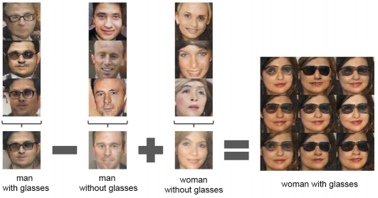
Here's a fun application of DCGANs for you - Vector Arithmetic using images of human faces. Yeah, you heard it right.

Implementing DCGAN on PyTorch

Before we get our hands dirty coding, let me give you a quick brief about the architecture of the generator and discriminator networks of a DCGAN.

The Discriminator model:

• Contains convolutional neural networks (CNNs) and Batch Normalization layers, alternating with each other.
• We use the Leaky ReLU activation function for all the layers except the final one, where we use the Sigmoid activation function (which squishes values to be between 0 and 1).

The Generator model:

• Contains tranposes of CNNs and Batch Normalization layers, alternating with each other.
• We use the ReLU activation function for all the layers except the final one, where we use the Tanh activation function (which squishes values to be between -1 and 1)

Let's proceed to code

I will follow a step-by-step procedure so it becomes easy for you to understand what is going on at every step, and so that you don't get lost.

Step 1: Importing the necessary libraries

import matplotlib.pyplot as plt
import itertools
import torch
import torch.nn as nn
import torch.nn.functional as F
import torch.optim as optim
import torchvision.datasets as dset
import torchvision.transforms as transforms

from torch.autograd import Variable
from torch.utils.data.dataset import Dataset

Step 2: Here, we will set the hyperparameters to be used during training

img_size = 64
n_epochs = 24
batch_size = 64
learning_rate = 0.0002

The learning rate parameter determines how quickly we want to proceed towards finding the global minima (in this case, how much we want the model to improve after every epoch).

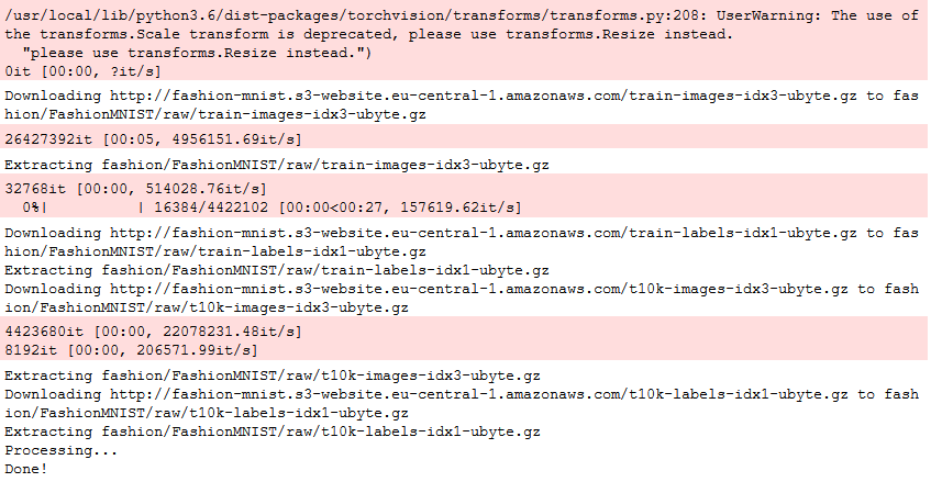
Step 3: For our model, we will use the Fashion-MNIST dataset and load it with the following code

transform = transforms.Compose([
    transforms.Scale(img_size),
    transforms.ToTensor(),
])

train_loader = torch.utils.data.DataLoader(
    dset.FashionMNIST('fashion', train = True, 
                      download = True, transform = transform),
    batch_size = batch_size,
    shuffle = True
)

Fashion-MNIST is an MNIST-like dataset of 70,000 28 x 28 labeled fashion images.

It shares the same image size and structure of training and testing splits.

You should see something like this in the output after you run the code above:

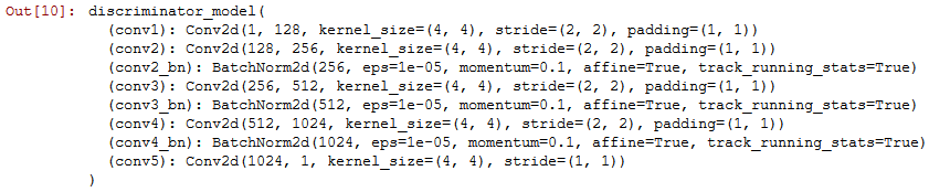
Step 4: Defining the discriminator network in a function

class discriminator_model(nn.Module):

  def __init__(self):
    super(discriminator_model, self).__init__()
    self.conv1 = nn.Conv2d(1, 128, 4, 2, 1)
    self.conv2 = nn.Conv2d(128, 256, 4, 2, 1)
    self.conv2_bn = nn.BatchNorm2d(256)
    self.conv3 = nn.Conv2d(256, 512, 4, 2, 1)
    self.conv3_bn = nn.BatchNorm2d(512)
    self.conv4 = nn.Conv2d(512, 1024, 4, 2, 1)
    self.conv4_bn = nn.BatchNorm2d(1024)
    self.conv5 = nn.Conv2d(1024, 1, 4, 1, 0)
    
  def weight_init(self):
    for m in self._modules:
      normal_init(self._modules[m])
      
  def forward(self, input):
    x = F.leaky_relu(self.conv1(input), 0.2)
    x = F.leaky_relu(self.conv2_bn(self.conv2(x)), 0.2)
    x = F.leaky_relu(self.conv3_bn(self.conv3(x)), 0.2)
    x = F.leaky_relu(self.conv4_bn(self.conv4(x)), 0.2)
    x = F.sigmoid(self.conv5(x))
    return x

Step 5: In Step 4, we have used the normal_init function, which we will be using in the generator as well. Let's define it.

def normal_init(m):
  if isinstance(m, nn.ConvTranspose2d) or isinstance(m, nn.Conv2d):
    m.weight.data.normal_(0.0, 0.02)
    m.bias.data.zero_()

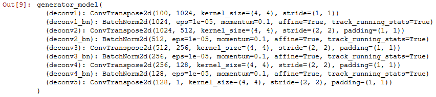
Step 6: Next, we define the generator

class generator_model(nn.Module):

  def __init__(self):
    super(generator_model, self).__init__()
    self.deconv1 = nn.ConvTranspose2d(100, 1024, 4, 1, 0)
    self.deconv1_bn = nn.BatchNorm2d(1024)
    self.deconv2 = nn.ConvTranspose2d(1024, 512, 4, 2, 1)
    self.deconv2_bn = nn.BatchNorm2d(512)
    self.deconv3 = nn.ConvTranspose2d(512, 256, 4, 2, 1)
    self.deconv3_bn = nn.BatchNorm2d(256)
    self.deconv4 = nn.ConvTranspose2d(256, 128, 4, 2, 1)
    self.deconv4_bn = nn.BatchNorm2d(128)
    self.deconv5 = nn.ConvTranspose2d(128, 1, 4, 2, 1)
    
  def weight_init(self):
    for m in self._modules:
      normal_init(self._modules[m])
      
  def forward(self, input):
    x = F.relu(self.deconv1_bn(self.deconv1(input)))
    x = F.relu(self.deconv2_bn(self.deconv2(x)))
    x = F.relu(self.deconv3_bn(self.deconv3(x)))
    x = F.relu(self.deconv4_bn(self.deconv4(x)))
    x = F.tanh(self.deconv5(x))
    return x

Step 7: To plot multiple random outputs during training, we create a function to plot the generated images

def plot_output():
  z_ = torch.randn((5*5, 100)).view(-1, 100, 1, 1)
  z_ = Variable(z_.cuda(), volatile = True)
  
  generator.eval()
  test_images = generator(z_)
  generator.train()
  
  grid_size = 5
  fig, ax = plt.subplots(grid_size, grid_size, figsize = (5, 5))
  for i, j in itertools.product(range(grid_size), range(grid_size)):
    ax[i, j].get_xaxis().set_visible(False)
    ax[i, j].get_yaxis().set_visible(False)
  for k in range(grid_size * grid_size):
    i = k // grid_size
    j = k % grid_size
    ax[i, j].cla()
    ax[i, j].imshow(test_images[k, 0].cpu().data.numpy(),
                    cmap = 'gray')
  
  plt.show()

Step 8: Let's create both networks by calling the defined functions, followed by initializing the weights

generator = generator_model()
discriminator = discriminator_model()
generator.weight_init()
discriminator.weight_init()

Step 9: Next, we need to make sure we use cuda

generator.cuda()

discriminator.cuda()

Step 10: For GANs, we can use the Binary CrossEntropy (BCE) loss function

BCE_loss = nn.BCELoss()

The purpose of a loss function is to calculate the difference between the actual output and the generated output.

Step 11: For both the networks, we need to set the optimizers with the following settings

beta_1 = 0.5
beta_2 = 0.999

G_optimizer = optim.Adam(generator.parameters(),
                         lr = learning_rate,
                         betas = (beta_1, beta_2))
                         
D_optimizer = optim.Adam(discriminator.parameters(),
                         lr = learning_rate / 2,
                         betas = (beta_1, beta_2))

Step 12: Final step! Now we can start training our networks with the following code block

for epoch in range(n_epochs):

  D_losses = []
  G_losses = []
  
  for X, _ in train_loader:
    discriminator.zero_grad()
    mini_batch = X.size()[0]
    
    y_real_ = torch.ones(mini_batch)
    y_fake_ = torch.zeros(mini_batch)
    
    X = Variable(X.cuda())
    y_real_ = Variable(y_real_.cuda())
    y_fake_ = Variable(y_fake_.cuda())
    
    D_result = discriminator(X).squeeze()
    D_real_loss = BCE_loss(D_result, y_real_)
    
    z_ = torch.randn((mini_batch, 100)).view(-1, 100, 1, 1)
    z_ = Variable(z_.cuda())
    G_result = generator(z_)
    
    D_result = discriminator(G_result).squeeze()
    D_fake_loss = BCE_loss(D_result, y_fake_)
    D_fake_score = D_result.data.mean()
    D_train_loss = D_real_loss + D_fake_loss
    
    D_train_loss.backward()
    D_optimizer.step()
    D_losses.append(D_train_loss)
    
    generator.zero_grad()
    
    z_ = torch.randn((mini_batch, 100)).view(-1, 100, 1, 1)
    z_ = Variable(z_.cuda())
    
    G_result = generator(z_)
    D_result = discriminator(G_result).squeeze()
    G_train_loss = BCE_loss(D_result, y_real_)
    G_train_loss.backward()
    G_optimizer.step()
    G_losses.append(G_train_loss)
    
  print('Epoch {} - loss_d: {:.3f}, loss_g: {:.3f}'.format((epoch + 1),
                                                           torch.mean(torch.FloatTensor(D_losses)),
                                                           torch.mean(torch.FloatTensor(G_losses))))
                                                           
  plot_output()

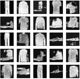
Here's the output of the first epoch:

And here's the output of the last epoch:

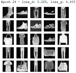
Isn't there a stark difference between the 2 images?

The image generated in the last epoch is more clearer and has less noise, than that generated in the first epoch.

So, we have learned about GANs, DCGANs and their uses cases, along with an example implementation of DCGAN on the PyTorch framework.

I hope you enjoyed reading this article, as much I did writing it !

In case you have any doubts, feel free to reach out to me via my LinkedIn profile and follow me on Github and Medium