
Hashing is the process of transforming data and mapping it to a range of values which can be efficiently looked up.
In this article, we have explored the idea of collision in hashing and explored different collision resolution techniques such as:
- Open Hashing (Separate chaining)
- Closed Hashing (Open Addressing)
- Liner Probing
- Quadratic probing
- Double hashing
-
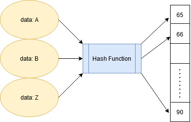
Hash table: a data structure where the data is stored based upon its hashed key which is obtained using a hashing function.
-
Hash function: a function which for a given data, outputs a value mapped to a fixed range. A hash table leverages the hash function to efficiently map data such that it can be retrieved and updated quickly. Simply put, assume S = {s1, s2, s3, ...., sn} to be a set of objects that we wish to store into a map of size N, so we use a hash function H, such that for all s belonging to S; H(s) -> x, where x is guaranteed to lie in the range [1,N]
-
Perfect Hash function: a hash function that maps each item into a unique slot (no collisions).
Hash Collisions: As per the Pigeonhole principle if the set of objects we intend to store within our hash table is larger than the size of our hash table we are bound to have two or more different objects having the same hash value; a hash collision. Even if the size of the hash table is large enough to accommodate all the objects finding a hash function which generates a unique hash for each object in the hash table is a difficult task. Collisions are bound to occur (unless we find a perfect hash function, which in most of the cases is hard to find) but can be significantly reduced with the help of various collision resolution techniques.
Following are the collision resolution techniques used:
- Open Hashing (Separate chaining)
- Closed Hashing (Open Addressing)
- Liner Probing
- Quadratic probing
- Double hashing
1. Open Hashing (Separate chaining)
Collisions are resolved using a list of elements to store objects with the same key together.
-
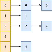
Suppose you wish to store a set of numbers = {0,1,2,4,5,7} into a hash table of size 5.
-
Now, assume that we have a hash function H, such that
H(x) = x%5 -
So, if we were to map the given data with the given hash function we'll get the corresponding values
H(0)-> 0%5 = 0 H(1)-> 1%5 = 1 H(2)-> 2%5 = 2 H(4)-> 4%5 = 4 H(5)-> 5%5 = 0 H(7)-> 7%5 = 2 -
Clearly 0 and 5, as well as 2 and 7 will have the same hash value, and in this case we'll simply append the colliding values to a list being pointed by their hash keys.
Obviously in practice the table size can be significantly large and the hash function can be even more complex, also the data being hashed would be more complex and non-primitive, but the idea remains the same.
This is an easy way to implement hashing but it has its own demerits.
- The lookups/inserts/updates can become linear [O(N)] instead of constant time [O(1)] if the hash function has too many collisions.
- It doesn't account for any empty slots which can be leveraged for more efficient storage and lookups.
- Ideally we require a good hash function to guarantee even distribution of the values.
- Say, for a load factor
λ=number of objects stored in table/size of the table (can be >1)
a good hash function would guarantee that the maximum length of list associated with each key is close to the load factor.
Note that the order in which the data is stored in the lists (or any other data structures) is based upon the implementation requirements. Some general ways include insertion order, frequency of access etc.
2. Closed Hashing (Open Addressing)
This collision resolution technique requires a hash table with fixed and known size. During insertion, if a collision is encountered, alternative cells are tried until an empty bucket is found. These techniques require the size of the hash table to be supposedly larger than the number of objects to be stored (something with a load factor < 1 is ideal).
There are various methods to find these empty buckets:
a. Liner Probing
b. Quadratic probing
c. Double hashing
a. Linear Probing
The idea of linear probing is simple, we take a fixed sized hash table and every time we face a hash collision we linearly traverse the table in a cyclic manner to find the next empty slot.
-
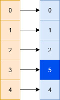
Assume a scenario where we intend to store the following set of numbers = {0,1,2,4,5,7} into a hash table of size 5 with the help of the following hash function H, such that
H(x) = x%5. -
So, if we were to map the given data with the given hash function we'll get the corresponding values
H(0)-> 0%5 = 0 H(1)-> 1%5 = 1 H(2)-> 2%5 = 2 H(4)-> 4%5 = 4 H(5)-> 5%5 = 0 -
in this case we see a collision of two terms (0 & 5). In this situation we move linearly down the table to find the first empty slot. Note that this linear traversal is cyclic in nature, i.e. in the event we exhaust the last element during the search we start again from the beginning until the initial key is reached.
- In this case our hash function can be considered as this:
H(x, i) = (H(x) + i)%N
where N is the size of the table and i represents the linearly increasing variable which starts from 1 (until empty bucket is found).
Despite being easy to compute, implement and deliver best cache performance, this suffers from the problem of clustering (many consecutive elements get grouped together, which eventually reduces the efficiency of finding elements or empty buckets).
b. Quadratic Probing
This method lies in the middle of great cache performance and the problem of clustering. The general idea remains the same, the only difference is that we look at the Q(i) increment at each iteration when looking for an empty bucket, where Q(i) is some quadratic expression of i. A simple expression of Q would be Q(i) = i^2, in which case the hash function looks something like this:
H(x, i) = (H(x) + i^2)%N
-
In general,
H(x, i) = (H(x) + ((c1\*i^2 + c2\*i + c3)))%N, for some choice of constants c1, c2, and c3 -
Despite resolving the problem of clustering significantly it may be the case that in some situations this technique does not find any available bucket, unlike linear probing which always finds an empty bucket.
-
Luckily, we can get good results from quadratic probing with the right combination of probing function and hash table size which will guarantee that we will visit as many slots in the table as possible. In particular, if the hash table's size is a prime number and the probing function is
H(x, i) = i^2, then at least 50% of the slots in the table will be visited. Thus, if the table is less than half full, we can be certain that a free slot will eventually be found. -
Alternatively, if the hash table size is a power of two and the probing function is
H(x, i) = (i^2 + i)/2, then every slot in the table will be visited by the probing function. -
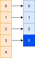
Assume a scenario where we intend to store the following set of numbers = {0,1,2,5} into a hash table of size 5 with the help of the following hash function H, such that
H(x, i) = (x%5 + i^2)%5.
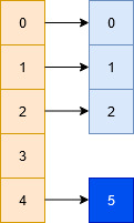
Clearly 5 and 0 will face a collision, in which case we'll do the following:
- we look at 5%5 = 0 (collision)
- we look at (5%5 + 1^2)%5 = 1 (collision)
- we look at (5%5 + 2^2)%5 = 4 (empty -> place element here)
c. Double Hashing
This method is based upon the idea that in the event of a collision we use an another hashing function with the key value as an input to find where in the open addressing scheme the data should actually be placed at.
- In this case we use two hashing functions, such that the final hashing function looks like:
H(x, i) = (H1(x) + i*H2(x))%N - Typically for
H1(x) = x%Na good H2 isH2(x) = P - (x%P), where P is a prime number smaller than N. - A good H2 is a function which never evaluates to zero and ensures that all the cells of a table are effectively traversed.
- Assume a scenario where we intend to store the following set of numbers = {0,1,2,5} into a hash table of size 5 with the help of the following hash function H, such that
H(x, i) = (H1(x) + i*H2(x))%5
H1(x) = x%5andH2(x) = P - (x%P), where P = 3
(3 is a prime smaller than 5)
Clearly 5 and 0 will face a collision, in which case we'll do the following:
- we look at 5%5 = 0 (collision)
- we look at (5%5 + 1*(3 - (5%3)))%5 = 1 (collision)
- we look at (5%5 + 2*(3 - (5%3)))%5 = 2 (collision)
- we look at (5%5 + 3*(3 - (5%3)))%5 = 3 (empty -> place element here)