Hashed Array Tree is an improvement over Dynamic Arrays where there can be a large amount of unused allocated memory at a time. This can be visualized as a 2 dimensional array and has been developed by Robert Sedgewick, Erik Demaine and others.

We will discuss:

1. Naive variable length arrays and why they don't work out?
2. What are dynamic arrays and how they work?
3. Problems with Dynamic Arrays
4. Idea of a new data structure
5. Concept of HAT
6. Inventor name and research paper
7. Time and Space Improvements with HATs
8. Conclusion
9. References

Naive variable length arrays and why they don't work out?

Arrays are the most widely used and a convenient data structure for a great many applications. They provide constant access time to their elements and are the structure of choice for many practical algorithms.

Appending an element to a variable length array is a common operation. The most naive (and the least efficient) approach is to increase the memory space reserved by the variable length array only when required, ie. one at a time.

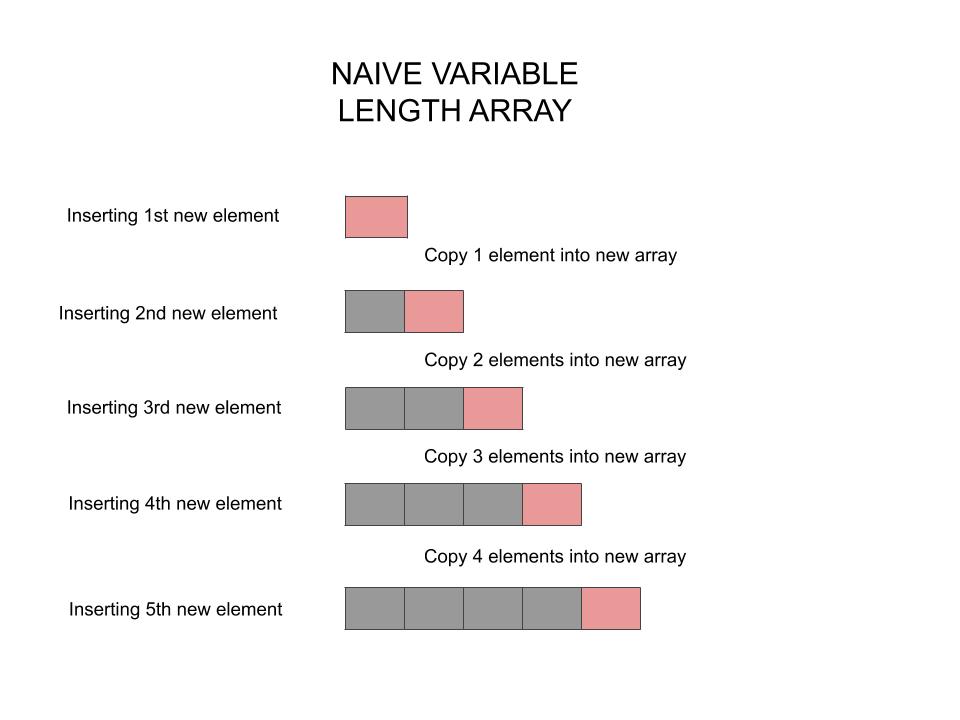
On doing this, we take up a lot many copying operations than is actually required.
As we can see in the above diagram, each new append will cost us $N$ copy operations of the $N$ elements to a new contiguous memory location (a new array) and $1$ insert operation of the new element.

For 4 appends to an array, we copy 10 elements $(1+2+3+4)$. If we calculate what it looks like, it stands to $N\frac{N+1}{2}$ copy operations and subsequent $N$ assignments, for appending $N$ elements to an array by this naive approach.

Which turns out to be $\mathcal{O}(n^2)$ algorithmically; and that just for appending a new element to an array! We can sort the array faster than that!

What are dynamic arrays and how they work?

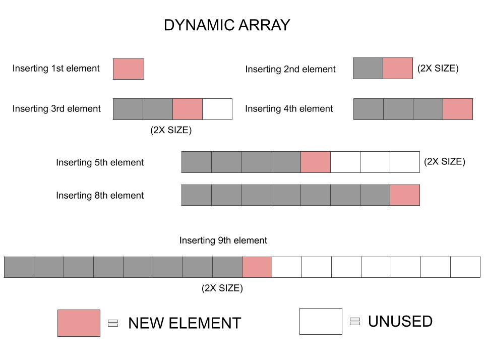
Dynamic Arrays work differently. When appending, it first checks whether the array is filled or not. If not, the new element is appended and that's all. Whereas if it is filled, it goes through the resizing procedure, where it copies all current elements to a new block of contiguous memory.

The difference from the naive approach is that the new contiguous block of memory does not include space for just one new element. In this approach the size of the newly allocated block of memory is increased to twice than that of the old one.

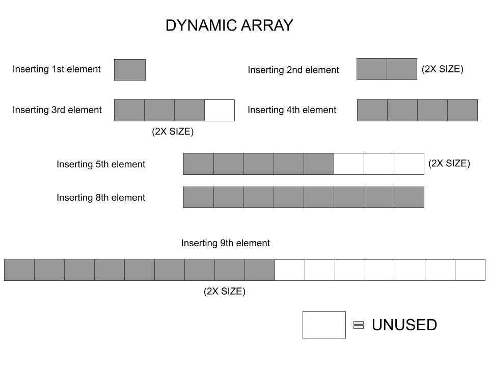
With this, there are lesser number of copy operations and not each append would need resizing all over again, as in the naive approach. We can see here that appending 9 elements to a dynamic array takes up only 15 (1+2+4+8) copying operations over only 4 resize cycles. We can go on and add 16 elements without any further resizing.

A quick calculation can tell us that since we need 15 copy operations to append 15 elements, we have managed to find a way to append new elements to a variable length array with a $\mathcal{O}(n)$ complexity, which is lots better than the naive approach. Also note, the number of assignments for the new elements do not increase.

Further, amortized analysis of the runtime for the insertion of an element at the end of such a structure would prove to be $\mathcal{O}(1)$.

So it's an improvement right? Not necessarily. It remains perfectly balanced, as all things should be. We'll talk about the tradeoff happening in this approach in the next section.

Problems with Dynamic Arrays

What we notice in the diagram is a lot of unused cells. And this increases as the array size grows larger.

This is where the Space-Time tradeoff happens. To make appending the new element more efficient we have sacrificed on the efficient utilization of space.

Consider a worst case situation where after inserting the 9th element, we do not ever need to insert any elements. That would leave 7 array cells empty. They cannot be utilized by any other part of the program as they are already a part of the array. This is nothing but wastage.

In the worst case, we see a space wastage of nearly $\frac{N}{2}$ blocks, where $N$ is the total space already allocated to the array. Which is written as an average of $\mathcal{O}(n)$ space wastage.

Idea of a new data structure

During the copy operation of arrays we've studied uptil here, BOTH the existing array and the new array must be present in memory at the same time, for elements to be copied from one to another whilst resizing.

This results in doubling the memory requirement of the array. Each time the array grows, it creates a memory fragment: the old array. This fragment becomes unusable the next time the array grows because the new array is larger and will not fit in the same memory space. This can increase the memory requirements by almost another factor of two.

But say we have a new data structure which somehow can improve on efficiency - in time and space. Let's see how!

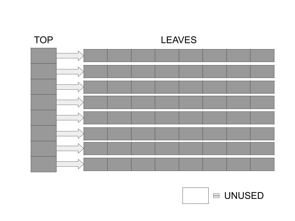
The following is a structure which consists of a single Top array and a number of Leaves which are pointed to by the elements in the Top array. The number of pointers in the Top array and the number of elements in each Leaf is the same, and is always a power of 2.

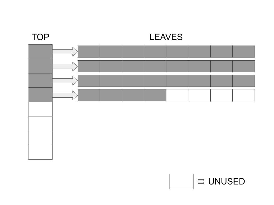
This is what it looks like diagrammatically. This one is a partially filled 8-HAT.

Concept of HAT

We store the one dimensional array into a structure that can be visualized in two dimensions. But doing so, we improve the problems we faced earlier with the naive variable length and the dynamic arrays. This new idea has been called Hashed Array Trees (or HATs).

Indexing

Because the Top and Leaf arrays are powers of 2, you can efficiently find an element in a HAT using bit operations.

power = log2(len(Top))
# for 16-HAT, power=4; for 8-HAT, power=3
top_index = needed_index >> power
leaf_index = needed_index & ((2**power) - 1);
# needed_index, top_index, leaf_index all are zero-based indices

Say for the 8-HAT example above, if we wanted to access value of array at index 26, without knowing how the implementation is done, we can access it via HAT_array[26] as normal. ALTHOUGH, there'll be functions in the background that process the actual result from the 2D structure.

The function would work as follows:

top_index = 26 >> 3  # 3
leaf_index = 26 & (8-1)  # 2
array_ele = HAT_2D_structure[top_index][leaf_index]
# return array_ele from function

Note: The same result can be easily achievable by performing division and modulo operation to calculate quotient and remainders, but bit operations are much faster, and that's the reason we have Top and Leaf always as powers of 2.

Appending

Usually, appending elements is very fast since the last leaf generally may have empty space; like we see in the example above. Less frequently, we'll need to add a new leaf, which is also very fast and requires no copying. We can add a leaf by creating a new empty array of the required size and have the next element from the Top array pointing to it.

When a HAT is full, copying and resizing cannot be avoided anymore. Here's an example of a completely filled 8-HAT:

The above structure has 64 elements in it, and is now ready to be resized before appending anything else in it.

This is when things get interesting. Sitarski's implementation first computes the correct size for the new HAT keeping in mind that the new Top and Leaf arrays are the same size, both a power of 2, then copies the elements into the new HAT structure, freeing the old leaves and allocating new leaves in an as needed basis.

For this particular example, the next power of 2 after 8 is 16. We'll have a new HAT which has a Top array of 16 elements and each of it's leaves will have 16 elements too. Only then, can we insert the 65th element to the HAT.

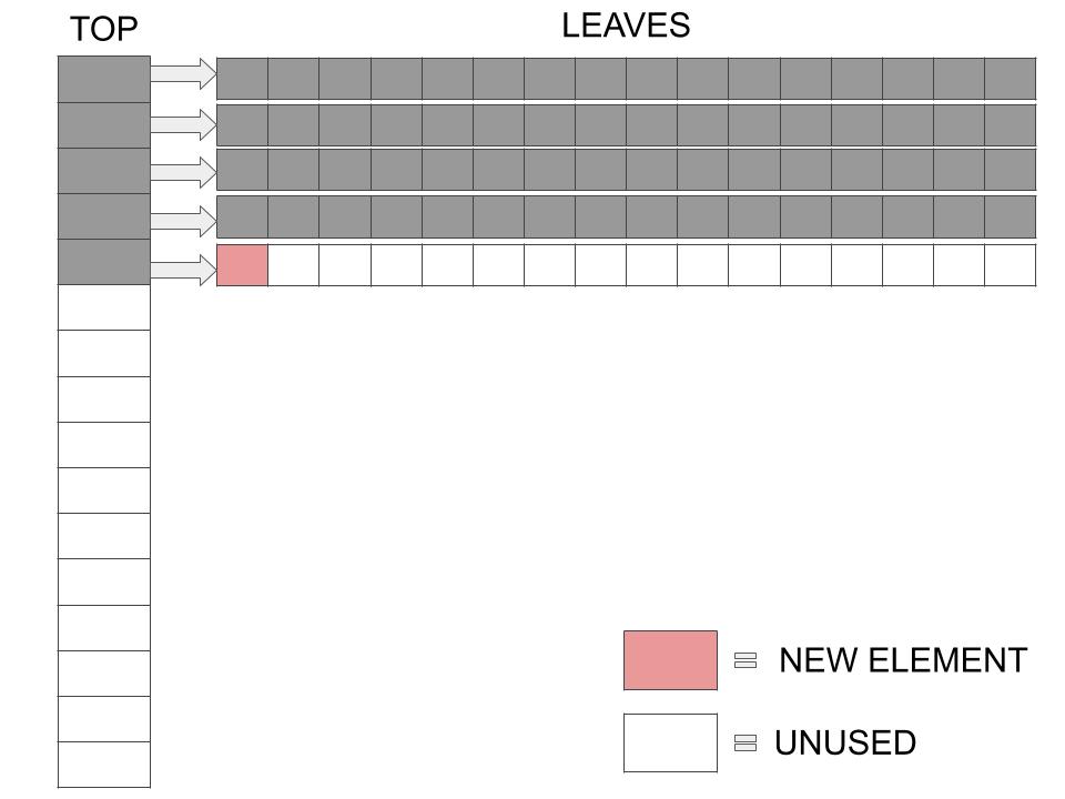
Inserting the 65th element above; which can be accessed at top[4][0], with zero-based indexing.

Inventor name and research paper

Sitarski Research Paper on HATs

Time and Space Improvements with HATs

1. TIME

• We can see here that once we undergo resizing for adding the 65th element, we won't have to undergo another resizing until after we reach the 256th element.
• Recopying occurs only when the Top array is full, and this happens when the number of elements exceeds the square of a power of 2 - rarely.
• The average number of extra copy operations is $\mathcal{O}(n)$ for sequentially appending $N$ elements like the dynamic array, unlike the naive variable length array's $\mathcal{O}(n^2)$.

2. SPACE

• The technique of reallocating and copying each leaf one at a time, when resizing, vastly reduces the memory overhead and the memory fragmentation is reduced.
• Unlike dynamic arrays, where BOTH the existing array and the new array had to be present in memory at the same time for copying, we do not need memory for a complete copy of the HAT.
• Memory is needed only for an extra new leaf. Morevoer, the leaf size depending on the square root of $N$ (total elements), the extra memory required during resizing decreases dramatically, as a percentage of N.

3. WASTAGE

• In the case of a 16-HAT, worst case of wastage occurs when we never append elements after the 65th element. Thus we can refer the diagram above and count the unused spaces remaining. A total of 15 cells remain unused in the new leaf. We assume the whole of the Top array to be unused as we do not actually use them to store any data, they're just used to point to the leaves. Thus we see the worst wastage of 31 (16+15) cells. (48% of data)
• As the HAT grows, the percentage of wasted memory in the worst case drops dramatically.
• Referring to this table from the research paper shows us exactly how much:
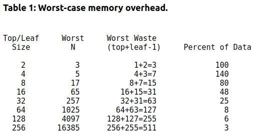
• The worst-case memory waste is $(top+leaf-1) \approx (2 * \sqrt{N}) \simeq \mathcal{O}(\sqrt{n})$. Which is so much better than an average of $\mathcal{O}(n)$ of the dynamic array.

Conclusion:

1. HATs are a practical and efficient way to implement variable-length arrays.
2. They offer highly desirable $\mathcal{O}(n)$ performance to append $N$ elements to an empty array.
3. Require only a $\mathcal{O}(\sqrt{n})$ memory overhead.
4. All the standard features and operations of a normal array are supported, including random access to elements.

	Array	Dynamic Array	Hashed Array Tree
Indexing	O(1)	O(1)	O(1)
Insert/delete at the beginning	N/A	O(n)	O(n)
Insert/delete at the end	N/A	O(1) amortized	O(1) amortized
Insert/delete at the middle	N/A	O(n)	O(n)
Wasted Space (Average)	0	O(n)	O(sqrt(N))

References:

1. Sitarski Research Paper
2. Brodnick Research Paper