In this article, we will discuss Image Compression application in depth involving Machine Learning Techniques like RNN based Encoder and Decoder and applications of Image Compression.

Table of Contents:

1. Introduction.
2. Image Compression
3. Need of Image Compression
4. Compression Techniques and Algorithm
   4.1 Lossless Compression
   4.2 Lossy Compression
5. RNN Based Encoder and Decoders for Image Compression.
   5.1 Types of Recurrent Units
   5.2 Reconstruction Framework
   5.3 Evaluation Metrics
6. Application of Image Compression.

Pre-requisites:

• Recurrent Neural Networks (RNN)
• Autoencoder
• Applications of Machine Learning

Introduction:

In recent years, the development and demand for multimedia products has accelerated, resulting in network bandwidth and memory device storage shortages. As a result, image compression theory is becoming increasingly important for minimising data redundancy and saving more hardware space and transmission bandwidth. In computer science and information theory, data compression or source coding is the process of encoding information using fewer bits or other information-bearing units than an unencoded representation. Compression is beneficial because it reduces the usage of costly resources like hard disc space and transmission bandwidth.

Compression focuses on reducing image size without sacrificing the uniqueness and information included in the original. The purpose of image compression is to eliminate image redundancy while also increasing storage capacity for well-organized communication.

Image Compression

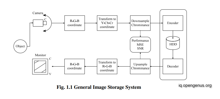
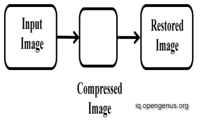
Image compression is a type of data compression in which the original image is encoded with a small number of bits. The goal of picture compression is to eliminate image redundancy and store or transfer data in a more efficient manner. The block diagram of the generic image storage system is shown in Figure 1.1. The fundamental purpose of such a system is to decrease the amount of data stored as much as feasible, so that the decoded image presented on the monitor is as close to the original as possible.

Now, let’s have a look at what is Image Compression Coding?

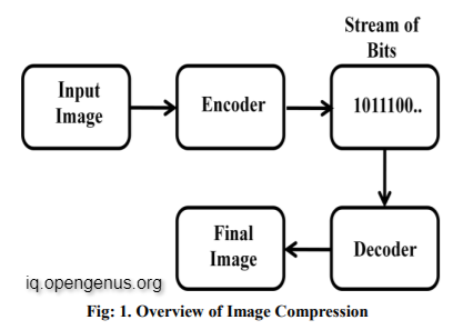
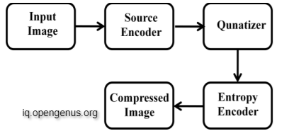
The goal of image compression coding is to save the picture as little as feasible in a bitstream and to display the decoded image as accurately as possible on the monitor. Consider the encoder and decoder depicted in Figure 1.2. When the encoder gets the original picture file, it converts it into a bit-stream, which is a sequence of binary data. The encoded bit-stream is subsequently received by the decoder, which decodes it to produce the decoded picture. Image compression occurs when the entire data quantity of the bit-stream is smaller than the total data quantity of the original image. Figure 1.2 depicts the whole compression flow.

The compression ratio is defined as follows:

			Cr = n1/n2

Pseudo code of the encoding algorithm:

    n ← the bit depth 
    Set the expectation value 
    While n > 0 { 
        Initialize the probabilities 
        for all pixels { 
            Define the context model, q 
            Binary arithmetic encoding of xn by q 
            Update the expectation value, y 
        }
         Output the code bit stream 
        n ← n − 1 
    }

Need of Image Compression

The raw data for single coloured photos does not require a lot of storage space. The overall storage needs become higher as the quantity of photos to be kept or images to be delivered grows. Uncompressed photos need more bandwidth for transmission and take longer to transmit, and if compressed before storage and transmission, the size of the image may be proportionate to its size. As a first stage, many forms of redundancy must be removed before compressing the photos. There are three main digital image redundancies that occur in most cases, and they are as follows:

1. Spatial Redundancy:
In the majority of natural photographs, the values of neighbouring pixels are tightly connected. Practically, the value of each given pixel may be anticipated based on the values of neighbouring pixels. This forecast based on a single pixel is less meaningful, and redundancy can be eliminated as a result. The wavelets transformation has the capacity to efficiently capture fluctuations at odd scales. As a result, these wavelets are ideal for this application.

2. Coding Redundancy:
When a picture is recorded as a matrix, the values range from 0 to 255, and this frequency distribution of pixel values is referred to as a histogram. It is simple to find repeated instances of each digit in the picture using this storage representation. When compared to other pixels, some pixel values have a higher frequency in typical photographs. When the same code word size is assigned to each pixel, coding redundancy is introduced. Huffman coding can help to minimise duplication. This is accomplished by allocating fewer bits to the additional grey scale values than to the less feasible bits.

3. Psycho visual Redundancy:
Psycho visual redundancy is based on human vision's features. Human eyes are unable to respond with equal sensitivity to all visual input. Psycho visual redundancy is a term used to describe how certain information is regarded as less important when compared to other information.

Compression Techniques and Algorithm

Compression is a procedure where particular information is characterized with reduced number of data points.

Compression Algorithm:

• The role of compression algorithm is to reduce the source of data to a compressed form and decompress it to get the original data.
• Any compression algorithm has two major components.
• • Modeler: It’s purpose is to condition the image data for compression using the knowledge of data.
• • Coder: encoder codes the symbols using the model while decoder decodes the message from the compressed data.

Compression Techniques:

Image compression techniques as shown in Figure and are broadly classified into two categories as lossy and lossless image compression.

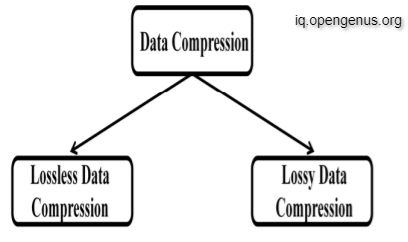
These two strategies are used to compress files and have the same goal. Lossy and lossless algorithms have distinct strategies for obtaining outcomes that are employed by different file formats. Discreet Cosine Transform, vector quantization, and Huffman coding are examples of lossy compression methods, whereas Run Length Encoding and string table are examples of lossless compression methods. The compression is measured by the compression ratio ( . Mathematically the quantity that measures the quality of a reconstructed image is compared with the original image and is known as peak signal to noise ratio (PSNR), that is measured in decides (dB).

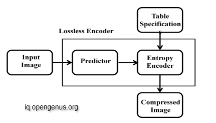
Lossless Compression:

This method is commonly used for archive purposes. Lossless compression is suggested for images with geometric forms that are relatively basic. It's used for medical, technical, and clip art graphics, among other things. The original data is totally recreated from the compressed data and utilised to size the file with no loss of image quality in this compression process, as illustrated in the Figure.

While compressing all the information in the original images is used. This will help in decompression to get back to original form that is accurately equal to the input data and the process is shown in the Figure.

Lossless compression may be utilised not only for graphic pictures, but also for computer data files like spreadsheets, text documents, and other software programmes like email attachments. A typical format is used to compress text files for repeated letters, and they are destroyed after a short period of time. The letters are recovered when the text file has been decompressed. Lossless compression algorithms have the benefit of being mostly helpful for compressing huge files. When recovering a file that has been compressed, the identical data is recovered following re-compression. After recompression, high-quality data is recovered, ensuring that the original and restored images are identical.

The main downside of Lossless Compression approaches is that the compression ratio will be low once the picture has been compressed. When data is compressed and sent, the time it takes to transport a picture is long. It's a challenging procedure to recreate a picture after it's been sent and decoded to obtain the original image back.

Different lossless compression Techniques:

1. Run Length Encoding:
Run length encoding is a lossless compression method that substitutes data with a pair of values: value, which represents the repeated value, and length, which represents the number of repeats. This is a basic compression technique that uses data in the form of runs. Runs are sequences in which the same data value appears in numerous data items in a row. Rather of storing the original run, they are saved as a single data value and count.

2. Predictive Coding:
This method uses the values of neighbouring pixels to anticipate the value of each pixel. As a consequence, instead of the original value, each pixel is encoded with a prediction error. When compared to the original value, these mistakes are much less, requiring fewer bits to record the data. Adaptive coding is a type of predictive coding that is similar to predictive coding. The picture is divided into blocks using this approach. The prediction coefficient is calculated on its own.

3. Arithmetic Encoding:
A message is represented by certain limited intervals between 0 and 1 in this encoding technique. The interval is broken into smaller intervals based on the probability of the message symbols. This method is the most capable at coding symbols based on the likelihood of their occurrence.

4. Entropy Encoding:
This method reduces the size of the dataset necessary to deliver a certain quantity of data. In Huffman and arithmetic coding approaches, the entropy coding method is applied. When characters and symbols appear repeatedly, they are first written down. Instead of repeating the process at each pixel, the locations of these pixels are recorded. The same symbols are applied to other people.

5. LZW Coding:
LZ technique replaces repetitive substrings to previous occurrences of strings. The repeated data is substituted by position and length of existing substring.

6. Huffman Coding:
Variable length coding is used in the Huffman Coding process.
Short code words are assigned to the most often used values or symbols in the data. Less frequently occurring values are assigned to longer code words. When compared to previous procedures, this methodology produces less redundancy cods. Text, pictures, and videos are compressed using this code.

Lossy Compression:

Lossy compression algorithms are very useful for compressing natural pictures such as photographs, where a small loss in reliability is sufficient to achieve a significant decrease in bit rate. This is the most common method for compressing multimedia data, and some data may be lost as a result. This is not suitable for text-based documents and applications, which require the exact information to be preserved without loss. Compared to lossless compression, this approach allows for a larger compression ratio. The reconstruction of a picture in this compression is simply an estimate of the original data, and the actual image is not returned as is, resulting in a very little amount of data loss, as illustrated in Figure.

This method of compression also looks for unnecessary pixel information, which is eliminated permanently. As a result, when the file is decompressed, the original data is not exactly returned. Data missing cannot be perceived even if the precise data is not retrieved. Figure depicts the lossy compression process.

Lossy compression algorithms have the benefit of being mostly helpful for compressing tiny files. When files are compressed, it takes much less time to transport them from one location to another, and they are much easier to move and store. These approaches produce files that are easy to use, open quickly, and are suitable for use in online applications. The processed files have a low resolution, low quality, and are usually threat-free.

Lossy compression algorithms have a number of drawbacks, one of which is that they do not allow for picture manipulation. The editable data is dumped in these pictures, which have a very low archive value. The processed photographs will have a poor resolution, which may compromise the quality of printing the images.

Different Lossy Compression Techniques:

1. Discrete Cosine Transform:
The Discrete Cosine Transform (DCT) is a lossy compression method for reducing picture and audio data. This method converts data into a sum of a sequence of cosine waves vibrating at various frequencies.

2. Discrete Wavelet Transform:
The picture is described as a sum of wavelet functions in the discrete wavelet transform. Wavelets are a type of function that has a different position and scale than other functions. This approach is usually used to picture blocks and is carried out using a hierarchical filter structure.

3. Fractal Compression:
This approach is based on the similarity of specific sections of a picture to other parts of the same image. This method transforms these elements into numerical data. Fractal codes are the data that is utilised to rebuild the encoded image. The image becomes resolution independent as it is turned into fractal code.

4. Vector Quantization:
This method uses the LBG-VQ algorithm, which is a fixed-length to fixed-length algorithm. It combines together a huge number of data points known as vectors. It converts values from a multidimensional vector space to a finite collection of values in a lower-dimensional discrete subspace. This reduced space vector requires less storage space and compresses data. This method is applied to both voice and visuals.

RNN Based Encoder and Decoders:

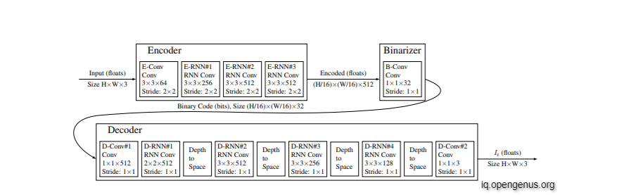
The recurrent units used to create the encoder and decoder include two convolutional kernels: one on the input vector which comes into the unit from the previous layer and the other one on the state vector which provides the recurrent nature of the unit. We will refer to the convolution on the state vector and its kernel as the “hidden convolution” and the “hidden kernel”.

In Figure, we give the spatial extent of the input-vector convolutional kernel along with the output depth. All convolutional kernels allow full mixing across depth. For example, the unit D-RNN#3 has 256 convolutional kernels that operate on the input vector, each with 3×3 spatial extent and full input-depth extent (128 in this example, since the depth of D-RNN#2 is reduced by a factor of four as it goes through the “Depth-to-Space” unit).

The spatial extents of the hidden kernels are all 1×1, except for in units D-RNN#3 and D-RNN#4 where the hidden kernels are 3×3. The larger hidden kernels consistently resulted in improved compression curves compared to the 1×1 hidden kernels.

Types of Recurrent Units:

1. LTSM:

Long short-term memory (LSTM) is an artificial recurrent neural network (RNN) architecture used in the field of deep learning. Unlike standard feedforward neural networks, LSTM has feedback connections. It can process not only single data points (such as images), but also entire sequences of data (such as speech or video). For example, LSTM is applicable to tasks such as unsegmented, connected handwriting recognition, speech recognition and anomaly detection in network traffic or IDSs (intrusion detection systems).

Let xt, ct, and ht denote the input, cell, and hidden states, respectively, at iteration t. Given the current input xt, previous cell state ct−1, and previous hidden state ht−1, the new cell state ct and the new hidden state ht are computed as:

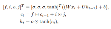
where ° denotes element-wise multiplication, and b is the bias. The activation function σ is the sigmoid function σ(x) = 1/(1 + exp(−x)). The output of an LSTM layer at iteration t is ht.

2. Associative LTSM:

An Associative LSTM combines an LSTM with ideas from Holographic Reduced Representations (HRRs) to enable key-value storage of data. HRRs use a “binding” operator to implement key-value binding between two vectors (the key and its associated content). They natively implement associative arrays; as a byproduct, they can also easily implement stacks, queues, or lists.

Associative LSTM extends LSTM using holographic representation. Its new states are computed as:

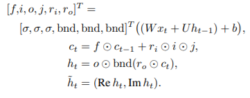
Associative LSTMs were effective only when used in the decoder.

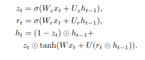
3. Gated Recurrent Units:

Gated recurrent units (GRUs) are a gating mechanism in recurrent neural networks, introduced in 2014 by Kyunghyun Cho et al. The GRU is like a long short-term memory (LSTM) with a forget gate, but has fewer parameters than LSTM, as it lacks an output gate. GRU's performance on certain tasks of polyphonic music modeling, speech signal modeling and natural language processing was found to be similar to that of LSTM. GRUs have been shown to exhibit better performance on certain smaller and less frequent datasets.

The formulation for GRU, which has an input xt and a hidden state/output ht, is

Reconstruction Framework:

In addition to using different types of recurrent units, we examine three different approaches to creating the final image reconstruction from our decoder outputs.

One-shot Reconstruction:

One-shot Reconstruction: As was done in Toderici et al. [2016], we predict the full image after each iteration of the decoder (γ = 0 in (1)). Each successive iteration has access to more bits generated by the encoder which allows for a better reconstruction. We call this approach “one-shot reconstruction”. Despite trying to reconstruct the original image at each iteration, we only pass the previous iteration’s residual to the next iteration. This reduces the number of weights, and experiments show that passing both the original image and the residual does not improve the reconstructions.

Additive Reconstruction:

In additive reconstruction, which is more widely used in traditional image coding, each iteration only tries to reconstruct the residual from the previous iterations. The final image reconstruction is then the sum of the outputs of all iterations (γ = 1).

Residual Scaling:

In both additive and “one shot” reconstruction, the residual starts large, and we expect it to decrease with each iteration. However, it may be difficult for the encoder and the decoder to operate efficiently across a wide range of values. Furthermore, the rate at which the residual shrinks is content dependent. In some patches (e.g., uniform regions), the drop-off will be much more dramatic than in other patches (e.g., highly textured patches).

To accommodate these variations, we extend our additive reconstruction architecture to include a content-dependent, iteration-dependent gain factor. Figure shows the extension that we used:

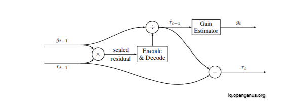
Adding content-dependent, iteration-dependent residual scaling to the additive reconstruction framework. Residual images are of size H×W×3 with three color channels, while gains are of size 1 and the same gain factor is applied to all three channels per pixel.

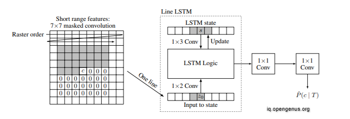
Binary recurrent network (BinaryRNN) architecture for a single iteration. The gray area denotes the context that is available at decode time.

Evaluation Metrics:

We use Multi-Scale Structural Similarity (MS-SSIM) a well-established metric for comparing lossy image compression algorithms, and the more recent Peak Signal to Noise Ratio - Human Visual System (PSNR-HVS). We apply MS-SSIM to each of the RGB channels independently and average the results, while PSNR-HVS already incorporates color information. MS-SSIM gives a score between 0 and 1, and PSNR-HVS is measured in decibels. In both cases, higher values imply a closer match between the test and reference images. Both metrics are computed for all models over the reconstructed images after each iteration. In order to rank models, we use an aggregate measure computed as the area under the rate-distortion curve (AUC).

Applications of Compression:

The above-mentioned Lossy Compression and Lossless Compression technologies are utilised for picture compression applications. Image compression programmes employ a variety of approaches and algorithms to compress pictures. The choice of one of these two approaches to compress photos is based on the quality of the output that the consumers anticipate. When consumers anticipate a very high quality output from image compression apps without any data loss, the programme might employ a lossless compression approach.

When a high level of precision is required, lossless compression methods are applied. The lossy compression approach can be utilised in some circumstances where the quality isn't as crucial and can be sacrificed. When this compression technique is applied, just a little amount of quality loss occurs, which is usually undetectable to the naked eye. It can be utilised in situations when a minor reduction in image quality is acceptable. Image compression is used in television broadcasting, remote sensing via satellite, military communication systems via radars, teleconferencing systems, computer-based communications systems, facsimile transmission medical images in computer tomography magnetic resonance imaging, capturing and transmitting satellite images, geological surveys, and weather reporting applications.

Some of the other applications are as follows:

• Broadcast Television
• Remote Sensing via satellite
• Tele Conferencing
• Medical Images
• Magnetic Resonance Imaging (MRI)
• Military Communications via radar,sonar.

With this article at OpenGenus, you must have the complete idea of