Problem: How can we improve on the convolution operators of CNNs?

Solution: Use of the Indirect Convolution algorithm

Explanation: It is a modification of GEMM-based algorithms

Indirect Convolution is as efficient as the GEMM primitive without the overhead of im2col transformations - instead of reshuffling the data, an indirection buffer is introduced (a buffer of pointers to the start of each row of image pixels). It can similarly support arbitrary Convolution parameters and leverage previous research on high-performance GEMM implementation.

Advantages:

• Outperforms the GEMM-based algorithm by up to 62% because it eliminates im2col transformations, which are expensive and memory-intensive. The benefits are most evident with a small number of output channels.
• Reduces memory overhead proportional to number of input channels due to the replacement of im2col buffers with smaller indirection buffer. The benefits are most evident with a small number of input channels.

Disadvantages:

• Optimised for NHWC layout, which is not competitive with path-building algorithms of Andersen et al due to strided memory access
• Minor performance reduction on 1x1 stride-1 convolutions
• Optimised for forward pass of convolution, so it ihas limited applicability for backward pass of a convolution operator
• It is inefficient for depthwise convolutions as they independently convolve their own set of features

Topic relevance:
50-90% of inference time in CNN models is spent in Convolution or Transposed Convolution operators

Background: Existing algorithms for 2D convolution operators

Direct convolution algorithm

Basic implementation:

• 7 nested loops iterating along batch size N, output height H_out, output width W_out, output channels K
• partial results accumulated across kernel heigh R, kernel width S and input channels C

Further modifications:

• extra loops for cache blocking
• vectorisation
  --> they complicate computation flow

Challenge: infeasible for a single implementation to deliver good performance across all parameter values with a standard layout for input and output tensors.

This implementation of Direct Convolution Algorithm as 7 nested loops is shown below.

for (int n = 0; n < N; n++)
   for (int oy = 0; oy < Hout; oy++)
       for (int ox = 0; ox < Wout; ox++)
           for (int oc = 0; oc < K; oc++)
               for (int ky = 0; ky < R; ky++)
                   for (int kx = 0; kx < S; kx++)
                       for (int ic = 0; ic < C; ic++) {
                           const int iy = oy * SY + ky * DY - PL;
                           const int ix = ox * SX + kx * DX - PT;
                           if (0 <= ix < Win && iy < Hin(
                               output [n][oy][ox][oc] += input[n][iy][ix][ic] * filter[oc][ky][kx][ic];
                               }

Modifications

1. Optimised direct convolution implementation
   Usage:

• Implemented in cuDNN and HexagonNN libraries, as well as MACE and ncnn frameworks
• For popular convolution parameters such as stride-2 kernels that are 5x1, 1x5 and 3x3
• A default algorithm for less common values is used

2. Parametrized architecture specific Just-In-Time code generator

• Product optimised direct convolution implementation
• Parameters are provided at runtime
• Further development: Autotuning is used for TVM in conjunction with the architecture

3. Use of specialised processor-specific layouts
   Challenges

• requires a large set of neural network operations
• costly layout conversions for convolution input/outputs

GEMM-based algorithms

Implementation:

• Computations in the Convolution operator are expressed as GEMM (matrix-matrix multiplication) operation, relies on im2col or im2row memory transformations
• Allows for use of BLAS (Linear Algebra) libraries - research can be used on every platform and benefit from previous research

Usage:

• All major deep learning frameworks, incl. TensorFlow, PyTorch, Caffe

Advantages:

• Support arbitrary parameters
• Generic implementation of Convolution operator

Fast Convolution Algorithms

Implementation:

• Use Fourier or Winograd transformation
• Reduce the computational complexity of Convolution with large kernel sizes (The asymptotic complexity of convolution doesn't depend on kernel size)
• Cannot be used as a default option as the speedup is limited to specific parameters - large kernel sizes, unit stride and dilation, adequately large input size, no. of input and output channels

Derivtion of the indirect convolution algorithm

The GEMM primitive computes the following equation

the implementation is as follows

    int k, const, float* pw,
    const float** pa, int lda,
    flat* pc, int ldc)
{
    const float* pa0 = pa;
    const float* pa1 = pa + lda;
    float c00 = 0, c01 = 0, c10 = 0, c11 = 0;
    do {
        const float a0 = *pa0++, a1 = *pa1++;
        const float *b0 = *pw++;
        c00 += a0 * b0;
        c10 += a1 * b0;
        const float b1 = *pw++;
        c01 += a0 * b1;
        c11 += a1 * b1;
        int kk = k;
        } while (--k != 0);
     pc[0] = c00; pc[1] = c01;
     pc += ldc;
     pc [0] = c10; pc[1] = c11;
  }

and can be represented in a figure

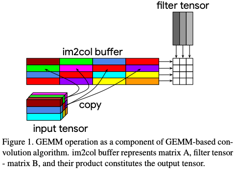
GEMM can be transfored to an Indirect GEMM by making two modifications. They allow the algorithm to implement a fused im2col + GEMM operation.

The implementation of the Indirect GEMM micro-kernel in C is as shown in the code below:

    int n, int k, const, float* pw,
    const float** ppa, int lda,
    flat* pc, int ldc)
{
    float c00 = 0, c01 = 0, c10 = 0, c11 = 0;
    do {
        const float *pa0 = *ppa++;
        const float *pa1 = *ppa++;
        int kk = k;
        do {
            const float a0 = *pa0++, a1 = *pa1++;
            const float b0 = *pw++;
            c00 += a0 * b0;
            c10 += a1 * b0;
            const float b1 = *pw++;
            c00 += a0 * b1;
            c10 += a1 * b1;
           } while (--kk != 0);
        } while (--n != 0);
     pc[0] = c00; pc[1] = c01;
     pc += ldc;
     pc [0] = c10; pc[1] = c11;
  }

It can be represented as such.

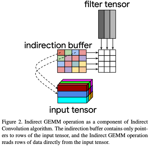
• Indirection buffers (pointers to rows of matrix A that are loaded from an array of pointers provided by the caller) specify the address of a row of pixels in the input tensor
• An extra loop is added over the elements of the kernel - one iteration loads new pointers to input rows from the indirection buffer, compute dot products of K elements as specified by the pointersand accumulate the results of the dot product

Indirection buffer is a buffer of pointers to rows of input pixels, with C pizels in each row and optionally strided. It depends on several parameters.

• Parameters of a neural network model are immutable
  • Parameters include convolution stride, dilation, kernel size, implicit padding, number of input channels, and output channels
• Complete re-initialisation of indirection buffer:
  • Changes in the height and width of input or output tensors
  • Changes in pointers to the input tenser/explicit zero factor - costs can be avoided by using a high-level framework to implement the convolution such that tenses have a persistent location regardless of shape changes
• Partial re-initialisation of the indirection buffer: changes in the batch size for batch indices not previously initialised

Definition of success

Success is defined by four factors:
Positive effect on performance

1. Elimination of im2col transformation for non-unit convolutions
2. Improvement in caching input rows for convolutions with large kernels
   Negative effect on performance
3. Overhead of loading points to rows of the input data from an direction buffer (point of comparison: computation under constant stride assumption)
4. Lower efficiency of two nested loops with RxS and C iterations (point of comparison: single loop with RxSxC iterations in the GEMM operation)

Variants of convolution implementation to be benchmarked are the (1) indirect convolution algorithm, (2) traditional GEMM-based algorithm and (3) the GEMM part of the traditional GEMM-based algorithm.

Experiment

Setup:

• Used 3 ARM64 Android devices
• Included high-performance and low-power cores
• Benchmarks were run in a single-threaded mode
  

Implementation

• GEMM and Indirect GEMM micro-kernels were used
  • Produced 4x8 output tile
  • Used same instruction sequence in the inner loop
• No need to repack (Goto, Van de Geijin) - as whole panels of A and B matrices read in the micro-kernel fit into level-1 cache, limited cache associativity is not a problem

Protocol

• Google Benchmark framework is used to take care of estimating sustained performance for the micro-benchmarks, which are repeated 25 times
• Micro benchmark run: cache state during neural network inference is simulated

Model

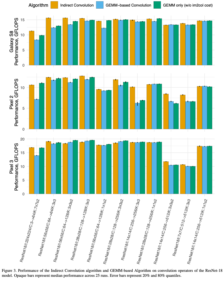
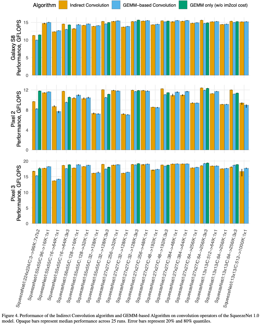
• Performance is evaluated on the convolution parameters of ResNet-18 and SqueezeNet 1.0
• Variety of convolution parameters are thus employed and yield a more balance experimental workload

The composition of convolution parameters in ResNet-18 and SqueezeNet 1.0 is shown below.

Results

The convolution algorithm has varying impact depending on the convolution parameters

• Convolutions with larger than 1x1 kernels see a performance improvement of 2.7-23.3%
• 1x1 stride-2 convolutions see an improvement of 0.5-8.0% (need im2col transformation in GEMM based algorithms but don't benefit from improved cache locality in the indirect GEMM)
• 1x1 stride-1 convolutions see a regression in performance of 0.3-1.9% (No im2col overhead is incurred, and the extra complexity in the Indirect GEMM primitive causes the regression - switching between GEMM or Indirect GEMM primitives can be better for overall performance)

The detailed results are shown in the following inmages for ResNet-18 and SqueezeNet 1.0 respectively.

The impact of these results on different types of convolution layers in the two models are shown below.

Analysis

Roofline model provides a consistent analysis tool for identifying the parameters with the greatest impact on performance. The indirect convolution algorithm is shown to be the most beneficial with a small number of output channels. The advantage of the indirect convolution algorithm grows with the system's arithmetic intensity.