
Get this book -> Problems on Array: For Interviews and Competitive Programming
Linear Regression is regression technique modelling relationship between dependent variable(y) and one or more independent variables(x) by using a linear approach. Usually when we solve a problem , we start by writing an function (such as y=mx+c) to map from independent variable to dependent variable . Then we provide input in order to get desired output. But in machine learning things are done differently. Here we have input values and we have output values, now we write an algorithm which gives a hypothesis function(h) which is a "good" predictor for the corresponding value of dependent variable(y) given independent variable(x).
To describe the linear regression problem more formally, our goal is given a training set, to learn a function h: x --> y , so that h(x) is a "good" predictor for the corresponding value of y.
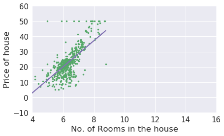
Let's understand this with an example. Suppose you have the dataset(Training set) of prices of house(Training variables), having features such as area of house, rooms in a house etc. and you have been asked to predict the price of the house provided these details. Now you have independent variables(x) as rooms,area etc. and you have to predict dependent variable y. Dependent variable is a variable whose value depends on other variables(independent variables). Now for such a large dataset it's hard to find out a function that's map between x and y. So, here comes linear regression, it finds the best possible (hypothetical) function to fit the data and then predicts the prices of any unseen house with the help of that function.
Linear Regression finds the parameters of that line which best fits the data, i.e., slope (theta1) and intercept (theta 0) in this case.
Gradient Descent
Gradient Descent is an optimization algorithm which we use to minimize cost function by repeating until convergence.
Cost Function
It tells us how good are model is at making predictions of the dependent variable(price of house) for the given set of parameters(theta1 and theta0). Cost function is basically the sum of squared difference of actual and predicted value. Minimum the value of cost function is better is our model at predicting values. So our goal is to minimize cost function.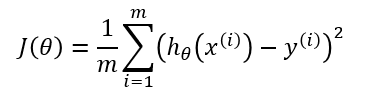
Now we can minimize cost function(get the local optima) with the help of gradient descent.We have two functions here h(x) and J(theta0,theta1), for different values of theta0,theta1 h(x) will have different values and there will be a graph for J(theta0,theta1) plotting different values. We want the global minima of that graph.When we plot for both theta0 and theta1 ,J(theta0,theta1) it forms a 3-D figure.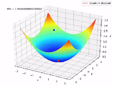
We will know that our model is accurate when our cost function is at the very bottom of the pits of the graph, i.e when its value is the minimum. The red arrow shows the minimum point in the graph.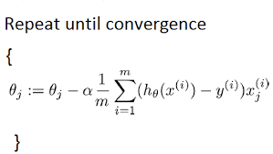
The way we do this is by taking the derivative(the tangential line to the function) of our cost function. The slope of the tangent is the derivative at that point and it will give us a direction in which we should we move in order to get reach minimum point. We make steps down the cost function in the direction with the steepest descent. The size of the each step is determined by the parameter α which is learning rate.
If you don’t know calculus, go to this page, actually we will find the slope of cost function w.r.t. theta1 and theta0 at particular values and will keep on subtracting that slope from theta1 and theta0 respectively. So that will make theta0 and theta1 shift the cost function more towards minimia after every iteration. Alpha(α) is learning rate i.e. how fast we want our parameters to be updated. Learning rate decides how big a step we take in order to reach the minimum point. If your learning rate is too small your model will take long time in training as it'll make tiny changes to your parameters(theta0,theta1). However your learning rate is set too high it may overshoot and model might never get to the minimum point. Most commonly used learning rate values are 0.1 or 0.01.
Let's Start Coding:
Importing important libraries:
import numpy as np
import matplotlib.pyplot as plt
import pandas as pd
Importing the Dataset:
#IMPORTING THE TRAIN DATASET
dataset = pd.read_csv ('train.csv')
X=dataset.iloc[:, :-1].values
y=dataset.iloc[:, 1].values
#IMPORTING THE TEST DATASET
dataset_test = pd.read_csv ('test.csv')
X_test=dataset_test.iloc[:, :-1].values
y_test=dataset_test.iloc[:, 1].values
Dataset will have two columns:
0    24  21.549452
1    50  47.464463
2    15  17.218656
3    38  36.586398
4    87  87.288984
..   ..        ...
995  71  68.545888
996  46  47.334876
997  55  54.090637
998  62  63.297171
999  47  52.459467

[1000 rows x 2 columns]
Let's have a look on features of our dataset:
dataset.describe()
Out[5]:
                 x            y
count  1000.000000  1000.000000
mean     50.241000    50.269484
std      28.838387    29.118060
min       0.000000    -3.839981
25%      25.000000    25.086279
50%      50.000000    49.904331
75%      74.250000    74.463198
max     100.000000   108.871618
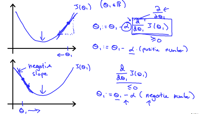
Let's visualize the dataset by plotting it on a 2-D graph to eyeball our dataset:
plt.scatter(X,y, color='blue')
plt.title('salary vs experience')
plt.xlabel('years of experience')
plt.ylabel('salary')
plt.show()
The above code will give us following plot.We have years of experience on x-axis and salary on y-axis.
finally, the time is to train our algorithm. For that, we need to import LinearRegression class, instantiate it, and call the fit() method along with our training data:
from sklearn.linear_model import LinearRegression
regressor = LinearRegression()
regressor.fit(X , y)
Now that we have trained our algorithm, it’s time to make some predictions. To do so, we will use our test data and see how accurately our algorithm predicts the percentage score. To make predictions on the test data, execute the following script:
y_pred = regressor.predict(X_test)
Now we'll compare the predicted value with the actual value of y:
df = pd.DataFrame({'Actual': y_test.flatten(), 'Predicted': y_pred.flatten()})
df
Output of the above commands


        Actual  Predicted
0    79.775152  77.155205
1    23.177279  20.890009
2    25.609262  21.894744
3    17.857388  19.885273
4    41.849864  35.961043
..         ...        ...
295  68.545888  71.126791
296  47.334876  46.008400
297  54.090637  55.051021
298  63.297171  62.084170
299  52.459467  47.013136


[300 rows x 2 columns]
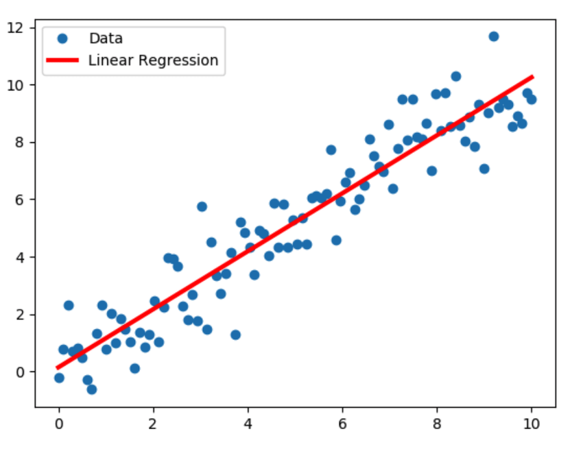
Let's look at how good our model do on our training set:
plt.scatter(X,y, color='blue')
plt.plot(X,regressor.predict(X),color='red')
plt.title('salary vs experience')
plt.xlabel('years of experience')
plt.ylabel('salary')
plt.show()
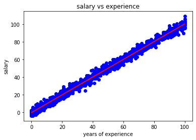
You can see that linear regression model have done quite a good work in finding the hypothesis function as our regressor fits well on our training set.But these were the values that model had already seen, let's see how good it predicts on test set:
plt.scatter(X_test,y_test, color='blue')
plt.plot(X,regressor.predict(X),color='red')
plt.title('salary vs experience')
plt.xlabel('years of experience')
plt.ylabel('salary')
plt.show()
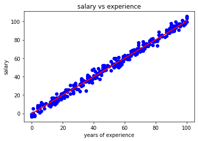
This shows that our model performed well even on the test set.The line fits pretty well on our test dataset. It pass right through the data.Thus, our model performs better on data that it has not seen previously. This shows how good our model is, we were able to generalize it.
Last step is to evaluate the performance of our algorithm. This step is important to see how different algorithms perform on a specific dataset. For regression algorithms most commonly used evaluation metrics is Mean Squared error(MSE). It's formula is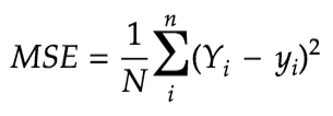
But we don't need to perform the calculation, we can use sklearn library function metrics to do it:
from sklearn import metrics
print('Mean Squared Error:', metrics.mean_squared_error(y_test, y_pred))
You'll receive following output:
Mean Squared Error: 9.294895563592618
As you can see Mean Squared Error is below 10% , it's quite good but we could make it better. This means our model can still make good predictions. We can make our model better by tweaking hyperparameters such as learning rate. You can play with them and see what gives good result for your dataset.