Connected Component Labeling, also known as Connected Component Analysis, Blob Extraction, Region Labeling, Blob Discovery or Region Extraction is a technique in Computer Vision that helps in labeling disjoint components of an image with unique labels.

This article covers the following topics:

1. What are Connected Components?
2. What is Connected Component Labeling?
3. Connected Component Labeling Algorithms.
4. Applying Connected Component Labeling in Python.

1. What are Connected Components?

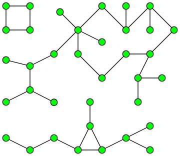
Connected Components or Components in Graph Theory are subgraphs of a connected graph in which any two vertices are connected to each other by paths, and which is connected to no other vertice in the supergraph.

The diagram below shows a graph with 3 Connected Components:

Connected Components in an image are set of pixels with the same value connected through Four Pixel Connectivity or Eight Pixel Connectivity.

Four Pixel Connectivity connects all pixels that have the same value along the edges.

Eight Pixel Connectivity connects all pixels that have the same value along the edges and corners.

Connected Components are used in Pattern Recognition, for Cluster Identification (Physics), identifying DNA Components (Biology) and in Social Network Analysis.

2. What is Connected Component Labeling?

Connected Component Labeling is used in computer vision using binary images to detect connected regions. Color images and higher dimensional data can also be used.

Connected Component Labeling solves the problem of finding out parts of the image that are connected physically, irrespective of color.
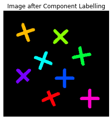
The Connected Components also known as Blobs can be counted, filtered and tracked. Below shown are a few examples of Connected Component Labeling:

3. Connected Component Labeling Algorithms:

Various methods can be used for Connected Component Labeling:

• Recursive Tracking (almost never used)
• Parallel Growing (needs parallel hardware)
• Row By Row (Most Common)
  • Classical Algorithm
  • Efficient Run Length Algorithm (developed for speed in industrial applications)

As the Classical Algorithm is the most commonly used method, it is explained in further detail below.

Classical Algorithm:

The Classical Algorithm is called so because it is based on the Alassical Connected Components Algorithm for graphs, was described in 1966, by Rosenfeld and Pfaltz. The algorithm makes two passes over the image:

• The first pass to record equivalences and assign temporary labels.
• Th second pass to replace each temporary label by the label of its equivalence class.

Before we delve into the steps involved in the algorithm we must understand the Union-Find Data Structure (Disjoint - Set Data Structure).

Union-Find Data Structure:

The Union-Find Data Structure keeps track of a set of elements divided into a number of disjoint subsets. It helps in efficiently implementing the following operations:

• Union: Join two subsets into a single subset.
• Find: Determine the subset the element is in.

The First Pass:

Each pixel is checked from the top left corner to the bottom right corner moving linearly. If we are considering the pixel p, we will check only the pixel above it and the pixel to the right.

Step 1:
The first step involves checking, if we are interested in a pixel or not. We are interested in foreground pixels, which in binary images are represented by a pixel value of 255 (White). If the image is not of interest we simply ignore it and move onto the next step.

Step 2:

In this step if we are interested in pixel p. We fetch the labels of the pixels above and to the left of p and store then A and B.

The following cases can arise:

• The pixels above or to the left or both are foreground pixels: Proceed as normal
• Both are background pixels: In this case, we create a new label and store it in A and B.

Step 3:

In this step we figure out which one out of A and B is smaller and assign that value to p.

Step 4:

If we have a situation where pixel above p has a label A and the pixel to the left of p has a label B. We know that these pixels are connected as pixel p connects them. Hence we need to store in information that the labels A and B are actually the same.

We do this by using the Union-Find Data Structure. We set the larger label as the child of smaller label.

Step 5:
Go to the next pixel.

The Second Pass:

In the second pass the algorithm goes through each pixel again and checks the label of the current pixel.

• If the label is a 'root' in the Union-Find Data Structure, it goes to the next pixel.

• If not it follows the links to the parent till it reaches the root after which it assigns that label to the current pixels.

The GIF image below demonstrates both the passes:

4. Applying Connected Component Labeling in Python:

Connected Component Labeling can be applied using the cv2.connectedComponents() function in OpenCV.

Below mentioned are steps:

Importing the libraries:

import cv2
import numpy as np
import matplotlib.pyplot as plt

Defining the function
The function is defined so as to show the original image and the image after Connected Component Labeling. The input the the function is the path to the original image.

def connected_component_label(path):
    
    # Getting the input image
    img = cv2.imread(path, 0)
    # Converting those pixels with values 1-127 to 0 and others to 1
    img = cv2.threshold(img, 127, 255, cv2.THRESH_BINARY)[1]
    # Applying cv2.connectedComponents() 
    num_labels, labels = cv2.connectedComponents(img)
    
    # Map component labels to hue val, 0-179 is the hue range in OpenCV
    label_hue = np.uint8(179*labels/np.max(labels))
    blank_ch = 255*np.ones_like(label_hue)
    labeled_img = cv2.merge([label_hue, blank_ch, blank_ch])

    # Converting cvt to BGR
    labeled_img = cv2.cvtColor(labeled_img, cv2.COLOR_HSV2BGR)

    # set bg label to black
    labeled_img[label_hue==0] = 0
    
    
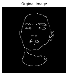
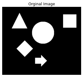
    # Showing Original Image
    plt.imshow(cv2.cvtColor(img, cv2.COLOR_BGR2RGB))
    plt.axis("off")
    plt.title("Orginal Image")
    plt.show()
    
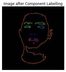
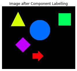
    #Showing Image after Component Labeling
    plt.imshow(cv2.cvtColor(labeled_img, cv2.COLOR_BGR2RGB))
    plt.axis('off')
    plt.title("Image after Component Labeling")
    plt.show()

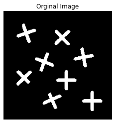
Passing in the image path in function

connected_component_label('C:/Users/Yash Joshi/OG_notebooks/shapes.png')

Output:

Other examples are mentioned in Section 2.

The complete code in a notebook format can be viewed here.

That wraps up this article, hope you found this article on Connected Component Labeling interesting and informative!

Further Readings

• Basics of Image Classification Techniques in Machine Learning by Harshit Kumar.
• Image Denoising and various image processing techniques for it by Nidhi Mantri.
• Build and use an Image Denoising Autoencoder model in Keras by Nidhi Mantri.
• Contrast Enhancement Algorithms by Yash Joshi