Pruning in Machine Learning is an optimization technique for Neural Network models. These models are usually smaller and efficient. Pruning aims to optimise the model by eliminating the values of weight tensors to gain computationally cost efficient model that takes less time in training.

Table of content:

1. Introduction to Pruning in ML
2. How to do Pruning?
3. Types of Pruning in ML
   3.1. Weight Pruning
   3.2. Unit pruning or Neuron pruning
   3.3. Iterative pruning
   3.4. Magnitude based pruning
4. Depth of Pruning
   4.1. Layer wise pruning
   4.2. Feature Map Pruning
   4.3. Kernel Pruning
   4.4. Intra Kernel Pruning
5. The idea of random pruning
6. Advantages of Pruning
7. Disadvantages of pruning

Introduction to Pruning in ML

Many algorithms like Convolutional Neural Networks suffer from the computational complexity issues. Hence we aim to find the most efficient way to for pruning the deep learning model and suggest a different approach for pruning.

Since the deep learning draws a lot of inspiration from human biology, the pruning is inspired from it too. In artificial neural networks the pruning is inspired from the human brain where the axons and dendrites completely decay and die in the beginning of the puberty years. This paper was titled "Optimal Brain Damage".

We can also prun the model from the very beginning. Pruning pipelines can be learned from the randomly initialised weights and channel importance iss learned by associating scalar gate values with each network layer.

Another method is Adversarial Neural Pruning combines the concept of adversarial training with the bayesian pruning methods.

The baysian pruning method is a standard convolutional neural network, the adversarial trained network, adversarial neural pruning, adversarial neural pruning with beta-bernoulli dropout, the adversarial trained network regurized with vulnerability supression loss and pruning network regularised with vulnerability supression loss.

The paper that gave rise to pruning was focused on the usage of theoretical information to derive practical and optimal ways to adapt the size of neural network. Removal of the unimportant weights from the network, many improvements were expected like:

• generalization
• fewer training examples
• better learning speed or classification speed.

The paper concluded that upon the reduction of the number of parameters in neural network by factor of four, additional factor of more than two was obtained by using optimal brain damage to delete the parameters automatically.

When we assume the objective function as the mean-squared-error, then the objective function increases when number of remaining parameters decreases.

To conclude, we can say that a "simple" network whose description needs small number of bits is more likely to generalize correctly as compared to more complex network as it has presumably already extracted essence of data and removed the redundancy.

How to do Pruning?

To perform the pruning we may follow the simple steps:

1. Build a simple network and train it
2. Measure the accuracy
3. Try pruning using various methodologies
4. Measure the accuracy and compare various models

The neural network resembles interconnection of neurons to the layer above it. We can even sort neurons according to their ranks.

Types of Pruning in ML

There are multiple types of pruning:

1. Weight Pruning
2. Unit pruning or Neuron pruning
3. Iterative pruning
4. Magnitude based pruning

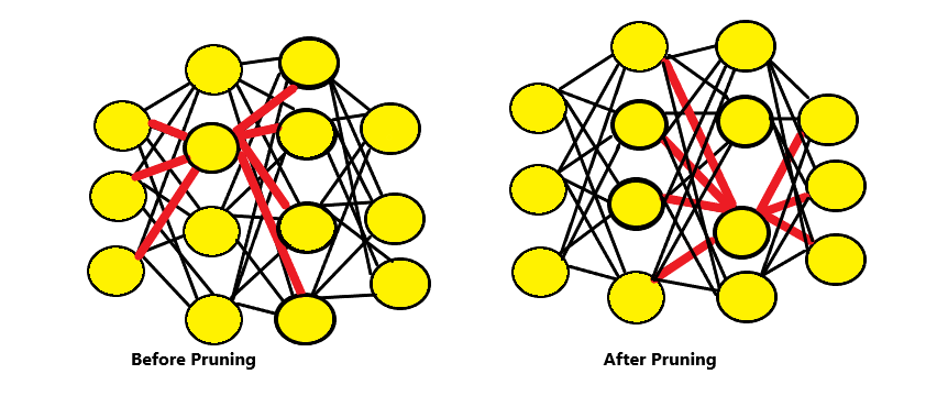
Weight Pruning

When we set the individual weights of the weight matrix to 0, we delete the connections. For example, to get sparsity of x percent, we would rank the individual weights in weight matrix according to their magnitudde. Then we would set the smallest x percent to zero.
To achieve the sparsity of k we would rank individual weights in weight matrix W according to their magnitude or absolute value. Then we set to zero the smallest k.

Unit pruning or Neuron pruning

In neuron pruning we would set all the columns to zero in the weight matrix to zero deleting the corresponding output neuron. Hence to achieve the sparsity of x percent, we rank the columns of a weight matrix and delete the smallest x percent.
Here to achieve sparsity of k we would rank the cloumns of a weight matrix according to their L2 - norm and delete the smallest k.

Iterative pruning

The iterative pruning refers to the iterative process of "Prun - Train - Repeat". The accuracy usually drops and to recover from it we use the "Prun - Train - Repeat" strategy. Over pruning can damage the network.

Magnitude based pruning

In the magnitude based pruning we consider the magnitude-based pruning. In this we consider the the magnitude of weight as a major criteria for pruning. Pruning is reducing the value of non-significant weights to zero.

We have 2 major options here:

• Given a trained network, prune it with more training
• We randomly take a network and then prune it from the scratch

There are multiple ways to optimise a neural-network based machine learning algorithms.

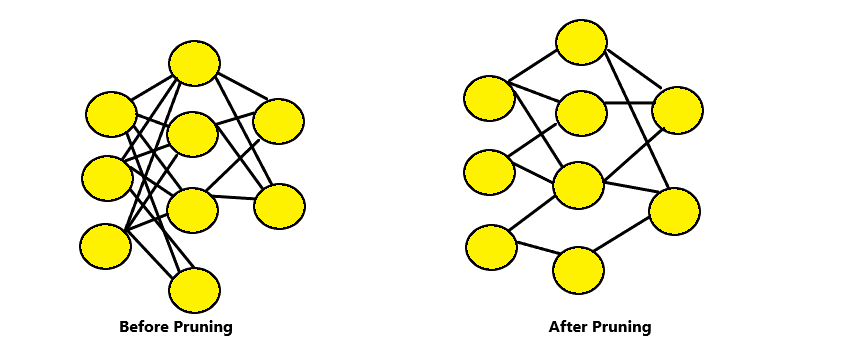
In the neural network before pruning, every neuron in the lower layer connects to the upper layer neuron. This eventually mean thaat we are required to multiply a lot of floats together. We ideally connect each neuron to other and then save it on doing multiplications. It is called "sparse" network.

Depth of Pruning

Layer wise pruning affects the depth of the network and a deep network can be converted into a shallow network. Increasing the depth improves the network performance and layer-wise pruning therefore demand intelligent techniques to mitigate the degradation of performance.

1. Layer wise pruning
2. Feature Map Pruning
3. Kernel Pruning
4. Intra Kernel Pruning

Layer wise pruning

The layer wise pruning technique, prunes the neurons layer by layer. It has shown to be more effective than pruning all neurons directly. Below illustration depicts the layer wise pruning. For each single layer pruning a corresponding 3 layer sub-network is extracted and we prune neurons in hidden layers. After we have performed pruning on one sub-network, we move to the next sub-network in sliding window fashion.

Feature Map Pruning

A feature map is a function that takes feature vectors in one space and transforms them into feature vectors in another. A feature map implicitly depends on the learning model class used and on the "input space" X where the data lies. Feature is a mapping of where a certain kind of feature is found in the image.

We can perform pruning on the feature maps. Feature map pruning removes a large number of kernels and may degrade the network performance much. We therefore may not achieve higher pruning ratios with this granularity. Feature map pruning affects the layer width and we directly obtain a thinner network and no sparse representation is needed.

Kernel Pruning

Kernel pruning is the next pruning granularity and it prunes k × k kernels. It is neither too fine nor too coarse. It is a balanced choice and the dense kernel connectivity pattern could be easily converted to a sparse one using it.

Each convolution connection involves width of feature map x height of feature map x kernel size x kernel size.

Intra Kernel Pruning

Intra kernel pruning technique eliminates the weights sructurally at an intra kernel level with original accuracy being retained. We need to conventionally train the neural network and set as the baseline before starting the pruning process. The trained network model is extracted and kernel that have similar locality are grouped into sets.

Pruning patterns indicate the locations at which parameters should be kept or eliminated. The Intra Kernel Pruning Involves, grouping kernels into sets.
For example, in 4 parameters, a 2 x 2 kernels is formed. The pruning follows thereafter.

The idea of random pruning

In randomized pruning, multiple pruning task are used in sequence one by one. The resulting sequence of expectation computations are averaged. The errors average on multiple computations. Time can be traded against the quality along with the errors of any single mask can be overcome.

The settings that make randomized pruning most advantageous are those in which programs that have a high-order dynamics can be vastly speeded by using masking.

Advantages of Pruning

• It reduces the size of decision trees by removing those parts of the tree which do not provide power for classifying instances.
• It is highly advantageous in removing the redundant rules which improve performance and sometimes accuracy too.

Disadvantages of pruning

• Whenever pruning tries to remove the repetitive rules, it sometimes affects the accuracy negatively.
• There is no single pruning technique that will always result in better perfromance and higher accuracy.
• The performance and accuracy are more dependent on the nature of the data.

Hence, pruning generally is useful for improving performance. However,for the sake of accuracy we need to do careful selections. No universal pruning technique can be classified as the best technique for accuracy and performace.

With this article at OpenGenus, you must have a strong idea of Pruning in Machine Learning.

Cite this article as:

Srishti Guleria. 
OpenGenus: Idea of Pruning in Machine Learning (ML) iq.opengenus.org/pruning-in-ml/.
Information available from iq.opengenus.org.
Accessed <add date>