In this article, we will be discussing a about RNN Based Encoder and Decoder for Image Compression.

Table of Contents:

1. Introduction.
2. Image Compression
3. RNN Based Encoder and Decoders
   3.1 Reconstruction Framework
   3.2 Entropy Encoding
   3.2.1 Single Iteration Entropy Coder
   3.2.2 Progressive Entropy Encoding
4. Evaluation Metrics

Pre-requisites:

• Image Compression: ML Techniques and Applications
• Image compression using K means clustering

Introduction:

The development and demand for multimedia goods has risen in recent years, resulting in network bandwidth and storage device limitations. As a result, image compression theory is becoming more significant for reducing data redundancy and boosting device space and transmission bandwidth savings. In computer science and information theory, data compression, also known as source coding, is the process of encoding information using fewer bits or other information-bearing units than an unencoded version. Compression is advantageous because it saves money by reducing the use of expensive resources such as hard disc space and transmission bandwidth.

Image Compression:

Image compression is a type of data compression in which the original image is encoded with a small number of bits. Compression focuses on reducing image size without sacrificing the uniqueness and information included in the original. The purpose of image compression is to eliminate image redundancy while also increasing storage capacity for well-organized communication.

There are two major types of image compression techniques:

1. Lossless Compression:
This method is commonly used for archive purposes. Lossless compression is suggested for images with geometric forms that are relatively basic. It's used for medical, technical, and clip art graphics, among other things.

2. Lossy Compression:
Lossy compression algorithms are very useful for compressing natural pictures such as photographs, where a small loss in reliability is sufficient to achieve a significant decrease in bit rate. This is the most common method for compressing multimedia data, and some data may be lost as a result.

RNN Based Encoder and Decoders:

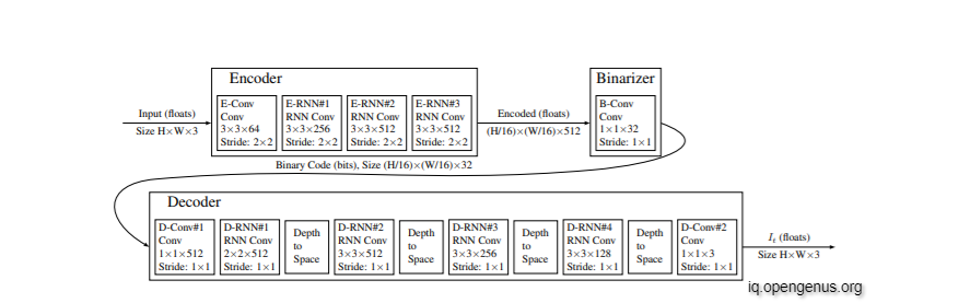
Two convolutional kernels are employed in the recurrent units used to produce the encoder and decoder: one on the input vector that enters into the unit from the previous layer, and the other on the state vector that gives the recurring character of the unit. The "hidden convolution" and "hidden kernel" refer to the convolution on the state vector and its kernel, respectively.

The input-vector convolutional kernel's spatial extent and output depth are shown in Figure. All convolutional kernels support full depth mixing. For example, the unit D-RNN#3 operates on the input vector with 256 convolutional kernels, each with 33 spatial extent and full input-depth extent (128 in this case, because D-depth RNN#2's is decreased by a factor of four when it passes through the "Depth-to-Space" unit).

Except in units D-RNN#3 and D-RNN#4, where the hidden kernels are 33, the spatial extents of the hidden kernels are all 11. When compared to the 11 hidden kernels, the larger hidden kernels consistently produced better compression curves.

Types of Recurrent Units:

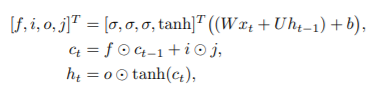
1. LTSM:
The long short-term memory (LSTM) architecture is a deep learning architecture that employs a recurrent neural network (RNN). LSTM features feedback connections, unlike standard feedforward neural networks. It is capable of handling not just single data points (such as images), but also whole data streams (such as speech or video). Tasks like unsegmented, linked handwriting identification, speech recognition, and anomaly detection in network traffic or IDSs (intrusion detection systems) can all benefit from LSTM.

Let xt, ct, and ht represent the input, cell, and hidden states at iteration t, respectively. The new cell state ct and the new hidden state ht are computed using the current input xt, prior cell state ct1, and previous hidden state ht1.

2. Associative LTSM:
To enable key-value storage of data, an Associative LSTM combines an LSTM with principles from Holographic Reduced Representations (HRRs). To achieve key-value binding between two vectors, HRRs employ a "binding" operator (the key and its associated content). Associative arrays are natively implemented as a byproduct. Stacks, Queues, or Lists can also be easily implemented

Associative LSTM extends LSTM using holographic representation. Its new states are computed as:

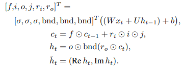
Only when employed in the decoder were associative LSTMs effective.

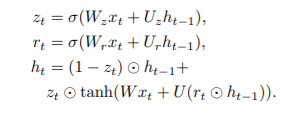
3. Gated Recurrent Units:
Kyunghyun Cho et al. established gated recurrent units (GRUs) as a gating technique in recurrent neural networks in 2014. The GRU is similar to a long short-term memory (LSTM) with a forget gate, but it lacks an output gate, hence it has fewer parameters. GRU's performance on polyphonic music modelling, speech signal modelling, and natural language processing tasks was found to be comparable to that of LSTM in some cases. On some smaller and less frequent datasets, GRUs have been found to perform better.

The GRU formula, which has an input xt and a hiddenstate/output ht, is as follows:

Reconstruction Framework:

Three distinct ways for constructing the final image reconstruction from the decoder outputs are explored, in addition to employing different types of recurrent units.

One-shot Reconstruction:

One-shot Reconstruction: As was done in Toderici et al. [2016], After each iteration of the decoder (= 0 in (1)), we predict the whole picture. Each cycle has more access to the encoder's produced bits, allowing for a better reconstruction. This method is known as "one-shot reconstruction." We merely transfer the previous iteration's residual to the next iteration, despite trying to rebuild the original picture at each iteration. The number of weights is reduced as a result, and trials demonstrate that sending both the original picture and the residual does not enhance the reconstructions.

Additive Reconstruction:

In additive reconstruction, which is more widely used in traditional image coding, each iteration only tries to reconstruct the residual from the previous iterations. The final image reconstruction is then the sum of the outputs of all iterations (γ = 1).

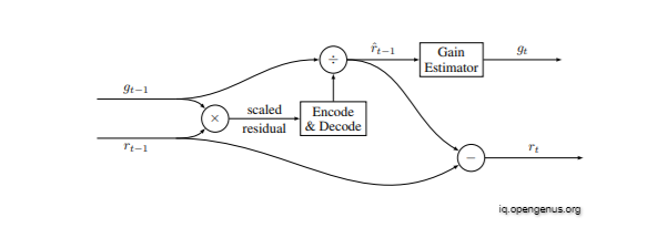
Residual Scaling:

The residual starts large in both additive and "one shot" reconstruction, and we anticipate it to diminish with each repetition. However, operating the encoder and decoder effectively across a large range of values may be problematic. In addition, the pace at which the residual diminishes is determined by the content. The drop-off will be significantly more apparent in certain areas (for example, uniform regions) than in others (e.g., highly textured patches).

The additive reconstruction architecture is enhanced to incorporate a content-dependent, iteration-dependent gain factor to address these variances.

The following is a diagram of the extension that is used:

Entropy Encoding:

Because the network is not deliberately intended to maximise entropy in its codes, and the model does not always utilise visual redundancy across a vast geographical extent, the entropy of the codes created during inference is not maximum. As is usual in regular image compression codecs, adding an entropy coding layer can boost the compression ratio even more.

The lossless entropy coding techniques addressed here are completely convolutional, process binary codes in progressive order, and process raster-scan order for a particular encoding iteration. All of our image encoder designs produce binary codes of the type c(y, x, d) with the dimensions H W D, where H and W are integer fractions of the picture height and width, and D is m the number of iterations. A conventional lossless encoding system is considered, which combines a conditional probabilistic model of the present binary code c(y, x, d) with an arithmetic coder to do the actual compression. More formally, given a context T(y, x, d) which depends only on previous bits in stream order, we will estimate P(c(y, x, d) | T(y, x, d)) so that the expected ideal encoded length of c(y, x, d) is the cross entropy between P(c | T) and Pˆ(c | T). We do not consider the small penalty involved by using a practical arithmetic coder that requires a quantized version of Pˆ(c | T).

Single Iteration Entropy Coder:

We employ the PixelRNN architecture for single-layer binary code compression and a related design (BinaryRNN) for multi-layer binary code compression. The estimate of the conditional code probabilities for line y in this architecture is directly dependent on certain neighbouring codes, but it is also indirectly dependent on the previously decoded binary codes via a line of states S of size 1 W k that captures both short and long term dependencies. All of the previous lines are summarised in the state line. We use k = 64 in practise. Using a 13 LSTM convolution, the probabilities are calculated and the state is updated line by line. There are three steps to the end-to-end probability estimation.

First, a 7/7 convolution is used to enlarge the LSTM state's receptive field, with the receptive field being the set of codes c(i, j, ) that potentially impact the probability estimate of codes c(y, x, ).

To prevent dependence on subsequent routines, this first convolution is a disguised convolution. The line LSTM in the second stage takes the output z0 of the initial convolution as input and processes one scan line at a time. The line LSTM captures both short- and long-term dependencies since LSTM hidden states are created by processing preceding scan lines. The input-to-state LSTM transform is likewise a masked convolution for the same reason. Finally, two 11 convolutions are added to the network to boost its capacity to remember additional binary code patterns. The Bernoulli-distribution parameter may be easily calculated using a sigmoid activation in the final convolution because we are attempting to predict binary codes.

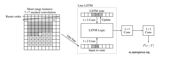
Above Image: Binary recurrent network (BinaryRNN) architecture for a single iteration. The gray area denotes the context that is available at decode time.

Progressive Entropy Encoding:

To cope with many iterations, a simple entropy coder would be to reproduce the single iteration entropy coder many times, with each iteration having its own line LSTM. However, such a structure would fail to account for the duplication that exists between iterations. We can add some information from the previous layers to the data that is provided to the line LSTM of iteration #k.

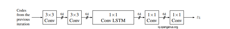
Description of neural network used to compute additional line LSTM inputs for progressive entropy coder. This allows propagation of information from the previous iterations to the current.

Evaluation Metrics

For evaluation purposes we use Multi-Scale Structural Similarity (MS-SSIM) a well-established metric for comparing lossy image compression algorithms, and the more recent Peak Signal to Noise Ratio - Human Visual System (PSNR-HVS). While PSNR-HVS already has colour information, we apply MS-SSIM to each of the RGB channels separately and average the results. The MS-SSIM score ranges from 0 to 1, whereas the PSNR-HVS is recorded in decibels. Higher scores indicate a closer match between the test and reference photos in both circumstances. After each cycle, both metrics are computed for all models across the reconstructed pictures. We utilise an aggregate metric derived as the area under the rate-distortion curve to rank models (AUC).

With this article at OpenGenus, you must have the complete idea of RNN Based Encoder and Decoder for Image Compression.