
Open-Source Internship opportunity by OpenGenus for programmers. Apply now.
In this article, we have explored the idea and computation details regarding pooling layers in Machine Learning models and different types of pooling operations as well. In short, the different types of pooling operations are:
- Maximum Pool
- Minimum Pool
- Average Pool
- Adaptive Pool
In the picture below, they both are cats! Whether sitting straight, or laying upside down. Being a cat is observed by observing their visual features and not the position of those features.
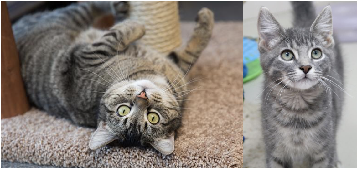
But often, convolutional layers, tend to give importance location of features. Pooling reduces that!
Pooling, progressively reduces the size of feature maps, introducing Translational Invariance.
Translational Invariance
Translational Invariance maybe defined as the ability to ignore positional shifts or translations in the target image.
It may also be referred to as decreasing spatial resolution to an extent that the exact location doesn't matter. Decreasing the importance of exact location enables a network to recognise local features to a certain degree.
A cat is still a cat, irrespective of its position!
NN(T(X)) = NN(X)
Let T() be a function the brings translational variance to a feature map X, the output after passing through the neural network NN() shall remain unchanged.
For this, sensitivity to location must be omitted. This is what pooling does.
For instance
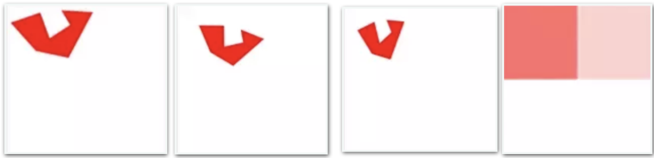
All the three images on the left, gives the same image on the right, The rotation and size of image doesn't matter, only the presence at the top left corner.
The exact position is discarded.
Above image might be interpreted as painting the entire area with the most pigmented colour. If you notice this, you are already versed with a famous pooling layer called the max-pooling layer.
Note: 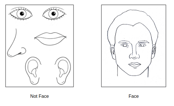
Above images, need to be distinguished too, the position isn't completely irrelevant, pooling needs to be conducted mindfully.
Any layer maybe defined by its hyperparameters.
Hyperparameters of a pooling layer
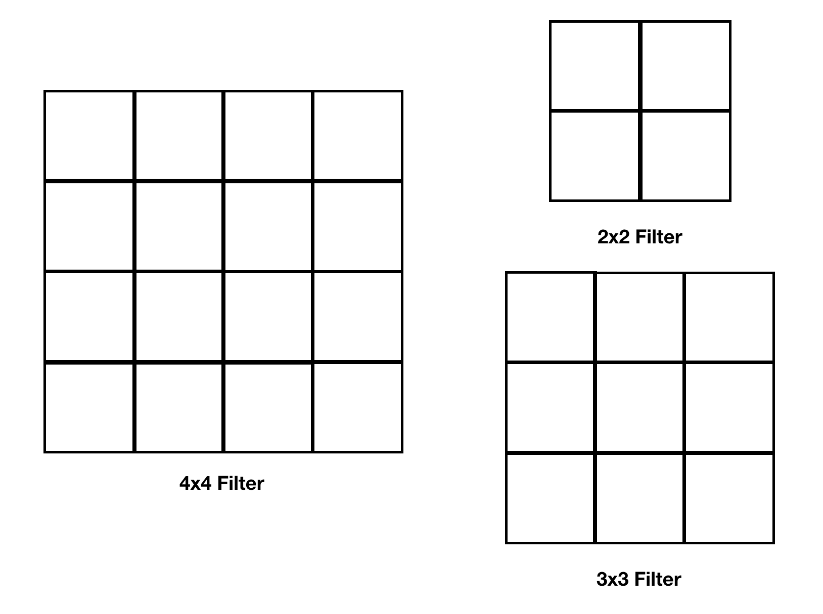
There are three parameters the describe a pooling layer
-
Filter Size - This describes the size of the pooling filter to be applied.
-
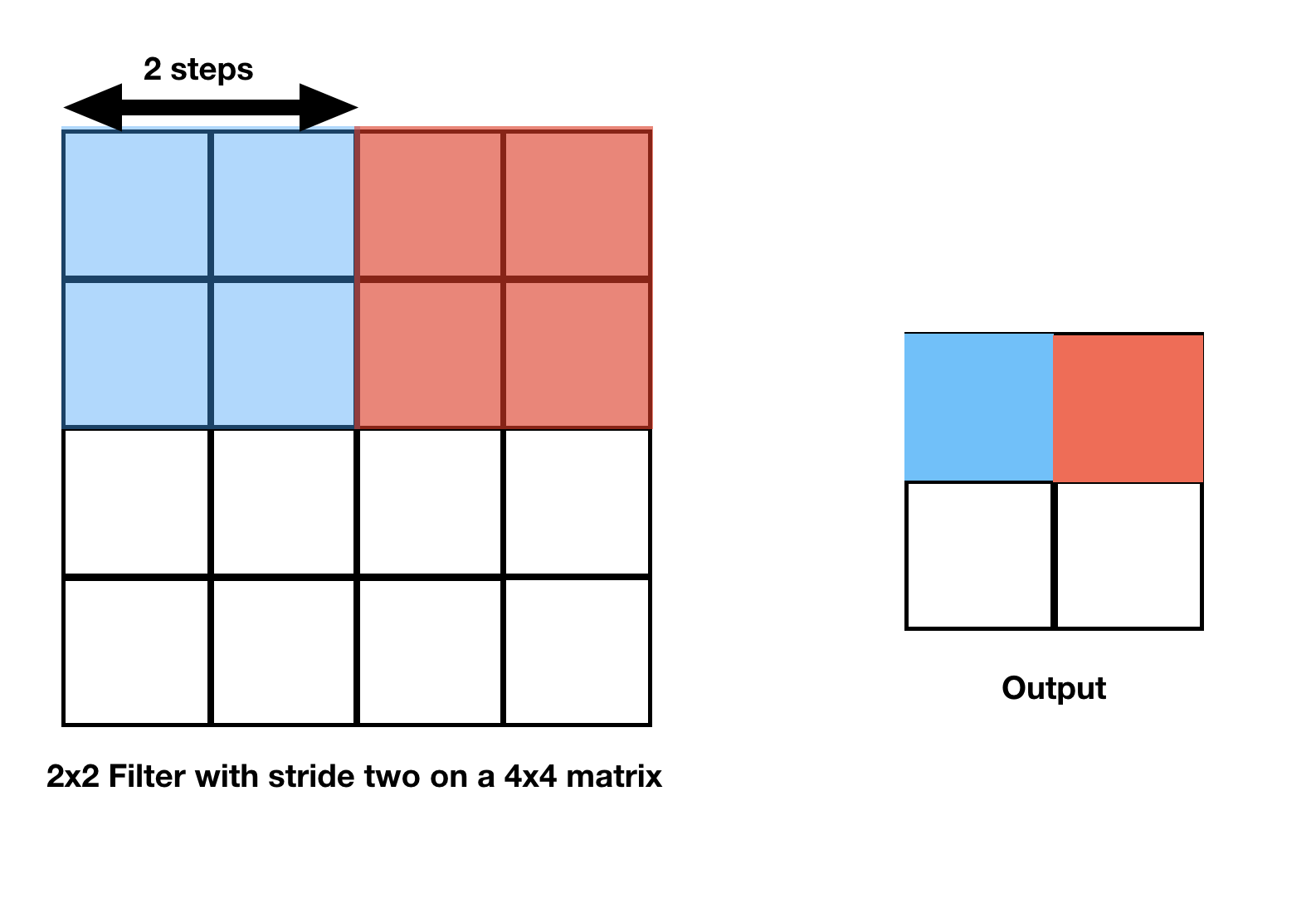
Stride - The number of steps a filter takes while traversing the image. It determines the movement of the filter over the image.
Examples
A filter with stride two must move two steps at a time.
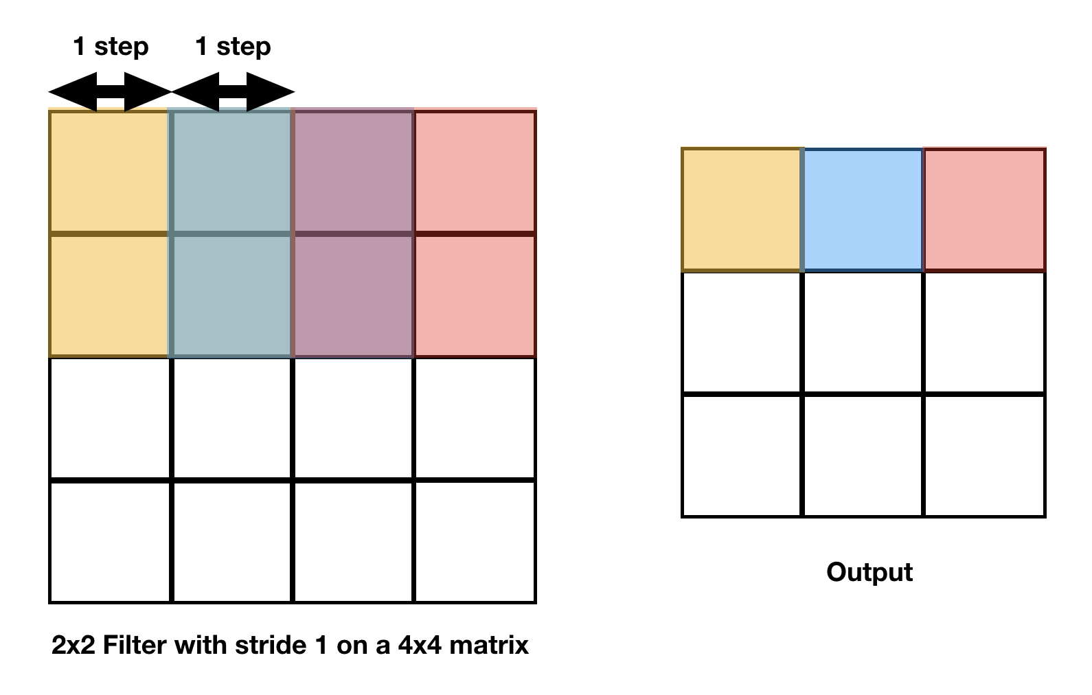
A filter with stride one must move one step at a time.
- Padding - Sometimes filter size creates a border effect in the feature map, the effect can be overcame through padding. This border effect refers to the fact that as a filter traverses a feature map, the border elemnts are generally much less used.
Also, the size of the image sets a limitation to how many times can an image be pooled, as pooling decreases the size.
Padding is done in such a situation, that is to add a border to our feature matrix.
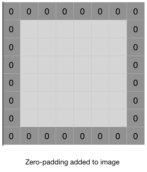
In this article, we will keep padding value as 0.
In the above example you may observe that a layer forms a smaller feature map, the fiter size is 3x3 and the stride is 1 i.e. it moves one step at a time.
The size of the resultant feature map maybe calculated by following formula.
where f = filter size ; p = padding ; s = stride
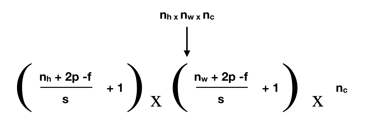
Above formula is for a three dimensional image wherein, the layer works on each slice of the volume.
Max Pooling
We saw the intuition of max pooling in the previous example. We're not sure though, whether the success of maxpooling is due to its intuitive approach or the fact that it has worked well in a lot of experiments.
It keeps the maximum value of the values that appear within the filter, as images are ultimately set of well arranged numeric data.
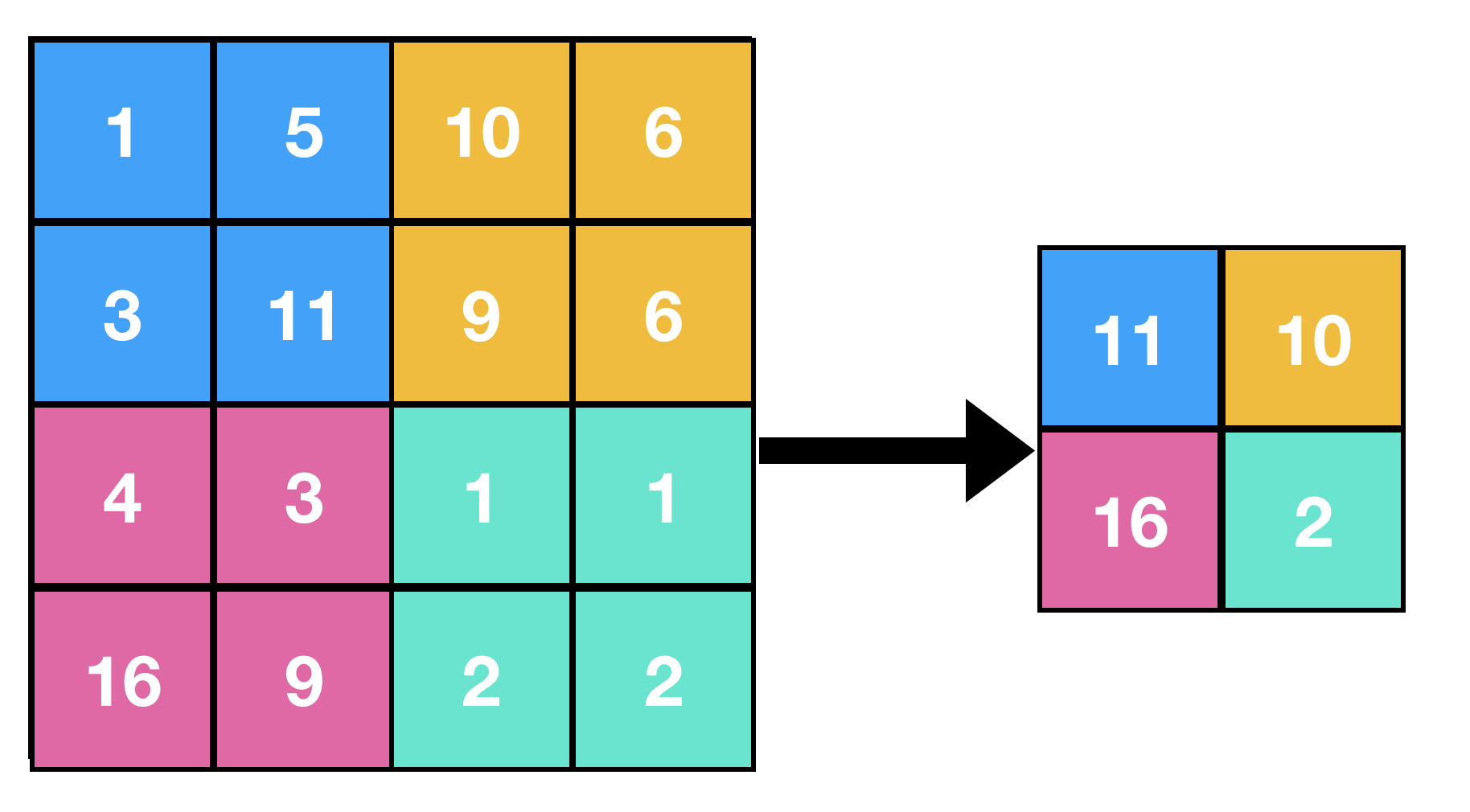
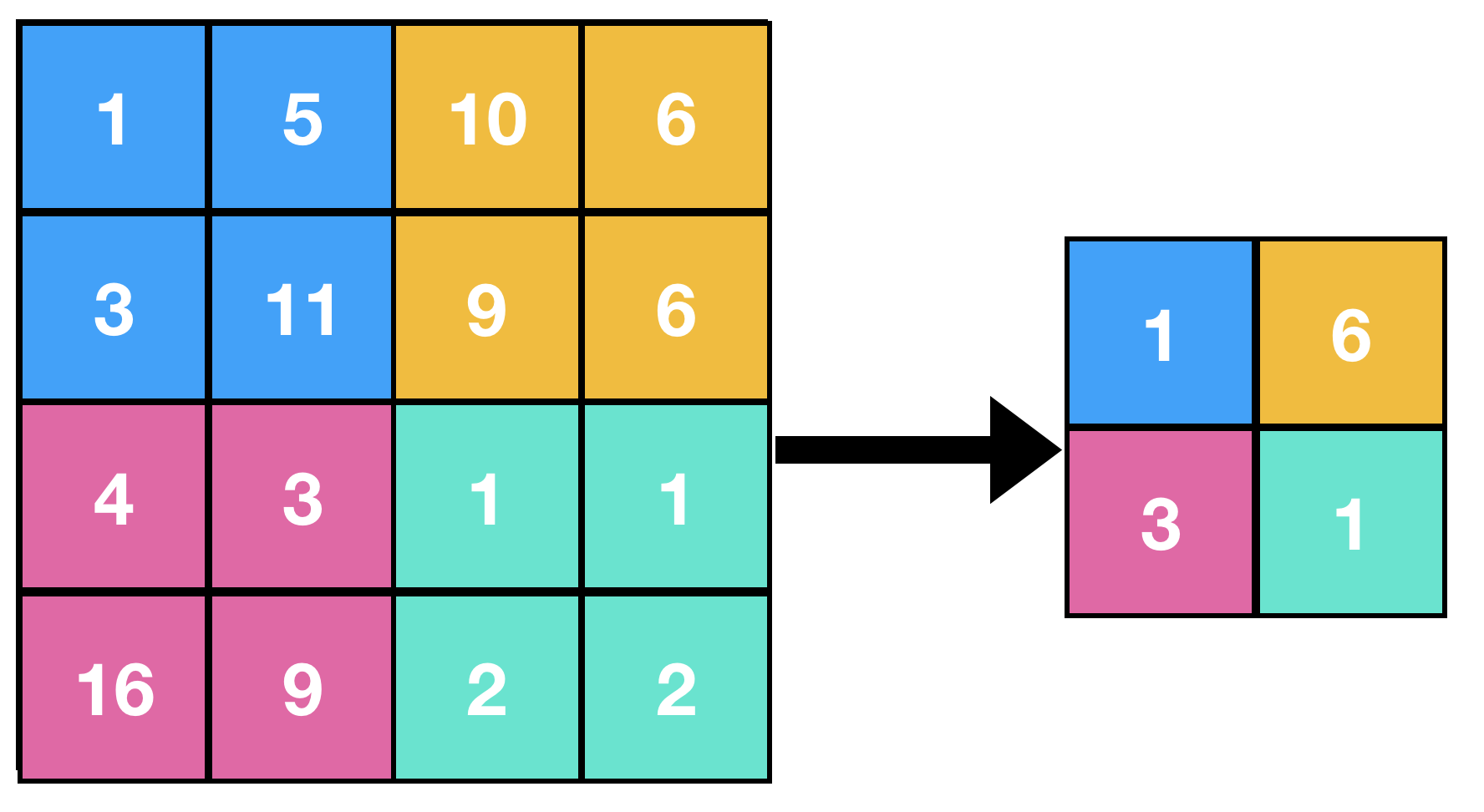
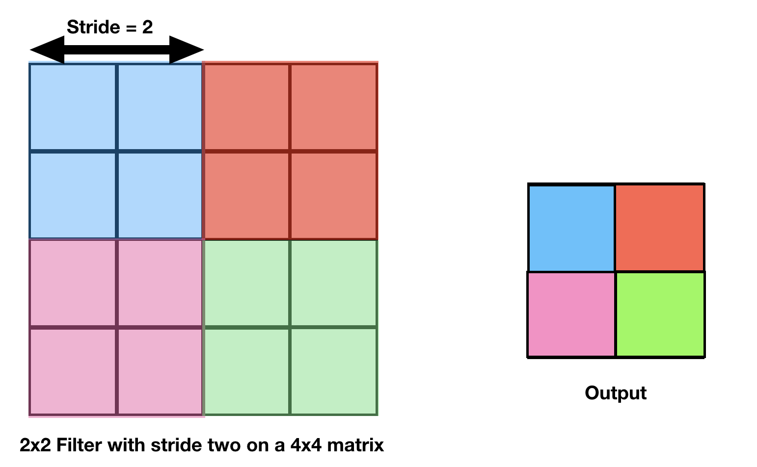
Below is an example of maxpooling, where
Filter size = 2
Stride = 2
Pseudocode
Here s = stride, and MxN is size of feature matrix and mxn is size of resultant matrix.
- Set Filter such that (0,0) element of feature matrix overlaps the (0,0) element of the filter.
- Set i=0 and j=0
- Obtain the maximum value amongst the values overlapped by the filter.
- Save the the value on the (i,j) position of resultant matrix.
- Increment j
- If j < n then: Move filter s steps forward and reapeat steps 3,4,5
- Else if i < m then: Increment i, move the filter such that (i,0) element of feature matrix overlaps (0,0) element of filter and Reapeat steps 3,4,5,6
Some of the general values of f and s are f = 3, s = 2 and f = 2, s = 2.
This is the Keras implementation of it
import numpy as np
from keras.models import Sequential
from keras.layers import MaxPooling2D
import matplotlib.pyplot as plt
# define input image
image = np.array([[1, 5, 10, 6],
[3, 11, 9, 6],
[4, 3, 1, 1],
[16, 9 ,2 ,2]])
#for pictorial representation of the image
plt.imshow(image, cmap="gray")
plt.show()
image = image.reshape(1, 4, 4, 1)
# define model that contains one average pooling layer
model = Sequential(
[MaxPooling2D (pool_size = 2, strides = 2)])
# generate pooled output
output = model.predict(image)
# print output image matrix
output = np.squeeze(output)
print(output)
# print output image
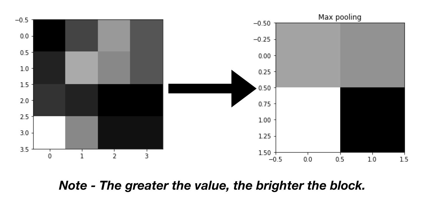
plt.imshow(output, cmap="gray")
plt.title('Max pooling')
plt.show()
Result
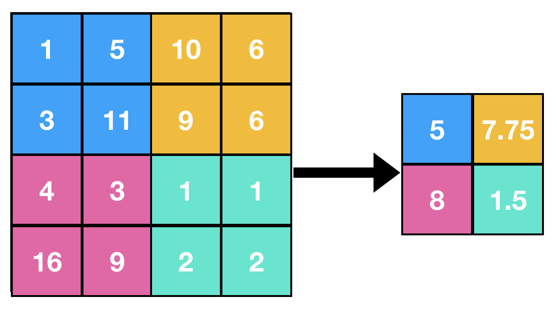
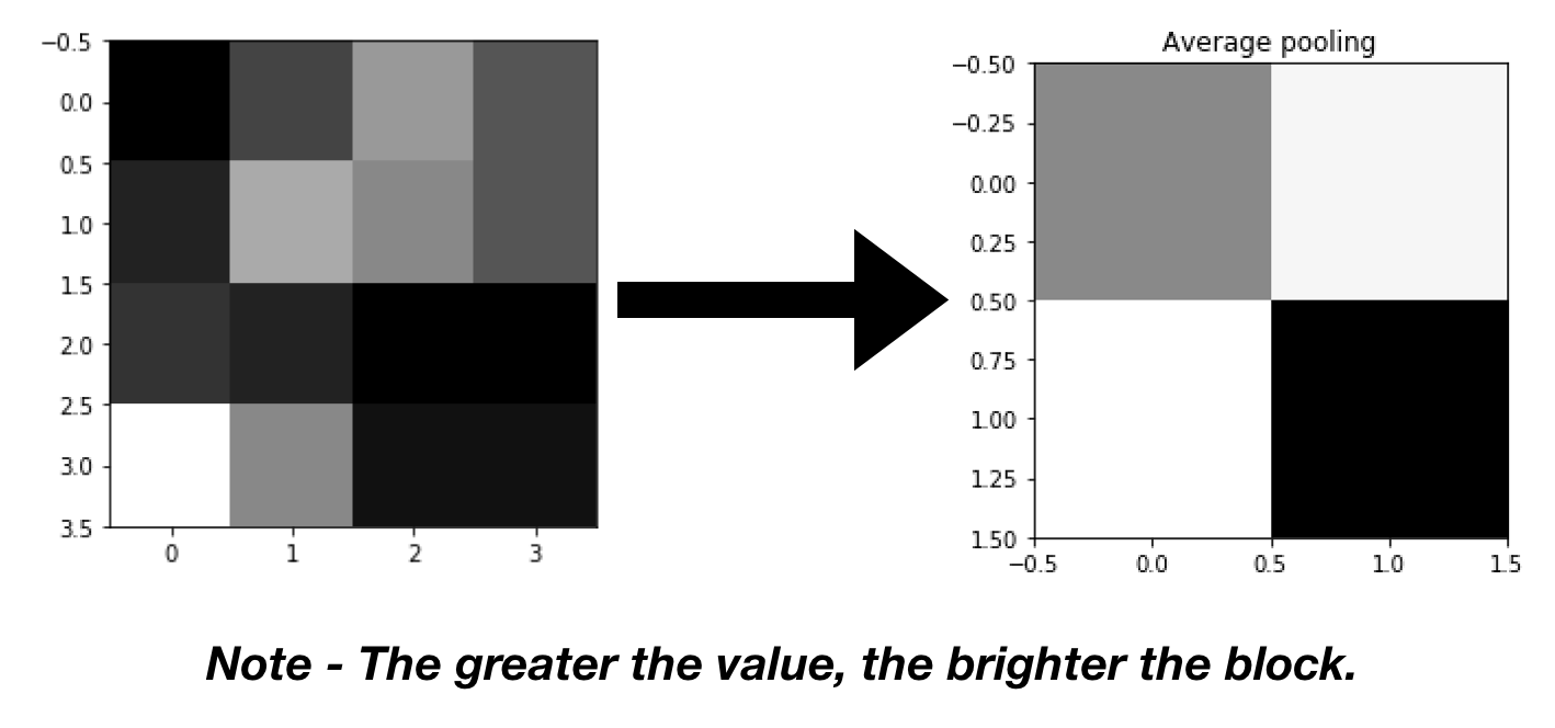
Average Pooling
This is used to collapse your representation. It removes a lesser chunk of data in comparison to Max Pooling.
It keeps the average value of the values that appear within the filter, as images are ultimately a set of well arranged numeric data.
Pseudocode
Here s = stride, and MxN is size of feature matrix and mxn is size of resultant matrix.
- Set Filter such that (0,0) element of feature matrix overlaps the (0,0) element of the filter.
- Set i=0 and j=0
- Obtain the average value of all the values overlapped by the filter.
- Save the the value on the (i,j) position of resultant matrix.
- Increment j
- If j < n then: Move filter s steps forward and reapeat steps 3,4,5
- Else if i < m then: Increment i, move the filter such that (i,0) element of feature matrix overlaps (0,0) element of filter and Reapeat steps 3,4,5,6
Keras has the AveragePooling2D layer to implement this.
Minimum Pooling
This is very similar to MaxPooling, here the minimum value is stored instead of the maximum one.
The idea must get clear by looking at our classic example.
Pseudocode
Here s = stride, and MxN is size of feature matrix and mxn is size of resultant matrix.
- Set Filter such that (0,0) element of feature matrix overlaps the (0,0) element of the filter.
- Set i=0 and j=0
- Obtain the minimum value amongst the values overlapped by the filter.
- Save the the value on the (i,j) position of resultant matrix.
- Increment j
- If j < n then: Move filter s steps forward and reapeat steps 3,4,5
- Else if i < m then: Increment i, move the filter such that (i,0) element of feature matrix overlaps (0,0) element of filter and Reapeat steps 3,4,5,6
Below image demonstrates the practical application of MinPooling.
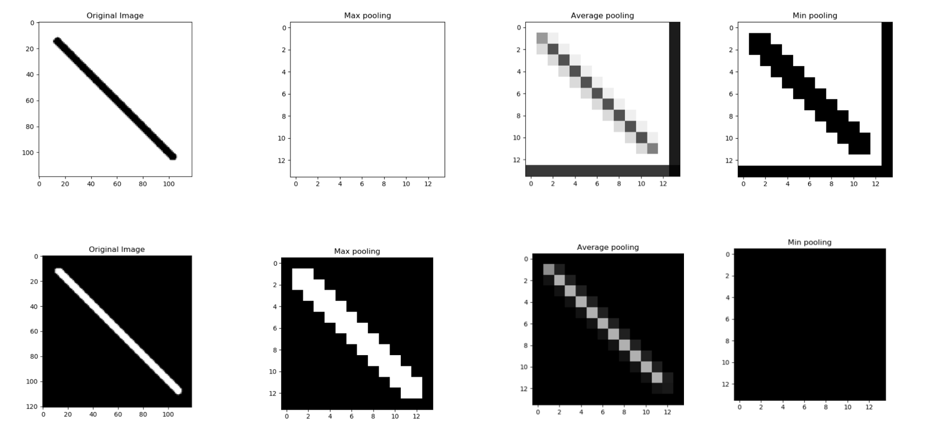
There are certain datasets where MinPooling could even triumph MaxPooling and we must be mindful for the same.
NOTE: References for maximum, minimum, average et cetera maybe taken globally too, as per requirement
Question
Which Hyper parameters does a Pooling layer need to be learnt while training?
Adaptive Pooling
A relatively newer pooling method is adaptive pooling, herein the user doesn't need to manually define hyperparameters, it needs to define only output size, and the parameters are picked up accordingly.
It is essentially equivalent to our previous methods, with different hyperparameters.
Example: Making these two Pytorch lines of code essentially equivalent
AvgPool2d(kernel_size = 2, stride = 2, padding = 0)
#Above the three parameters ensure that the output is 2 x 2
nn.AdaptiveAvgPool2d(2)
#Here instead of specifying the kernel_size, stride or padding. Instead, we specified the output dimension i.e 2 x 2
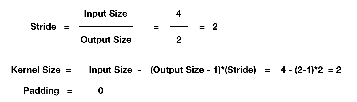
Herein, the layer adapts according to the output size specified, through the determined pooling method. The formulae can be inversely generated from the pooling formula.
Below is the formula and calculation for the case drawn just after the formula.
These are some major pooling layers.
Below is how you CNN probably looks like, and where does your pooling layer fit in.
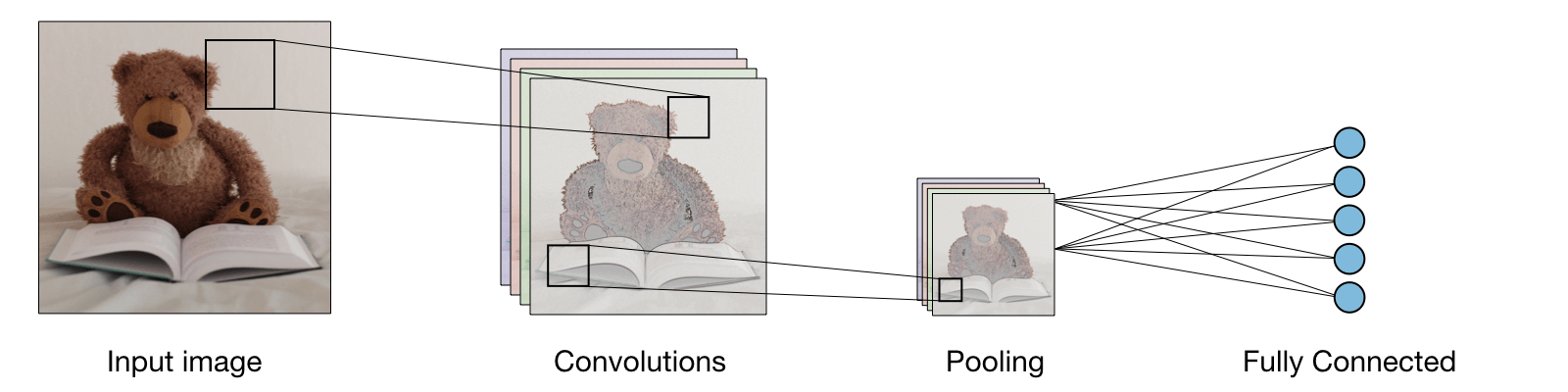
Now that you have a clear understanding of pooling and its major types. It is your turn to explore more, and build your CNN efficiently!
Wanna did deeper?
- MaxPool vs AvgPool layers in Machine Learning models by Priyanshi Sharma at OpenGenus
- Purpose of different layers in Machine Learning models by Priyanshi Sharma at OpenGenus
- List of Machine Learning topics at OpenGenus
- This is how Pooling layers are implemented in Keras library
With this article at OpenGenus, we must have a complete idea of pooling layers in Machine Learning. Enjoy.