Understanding Convolutional Neural Networks through Image Classification

Reading time: 30 minutes | Coding time: 15 minutes

Ever wondered how cool it would be if the retail stores can provide us with real-time shopping experience by analyzing and classifying our emotions.
Well, this is already happening, thanks to the power of deep learning and AI, which makes the core concepts of computer vision work so well.

The idea of classifying our emotions in the case above comes under image classification, which finds a place in almost every computer vision task.

Other famous applications of image classification include facebook auto-tagging feature, detection and classification of pedestrians and cars in self-driving cars, disease classification using X-ray images, and of course, the much-debated hotdog/not-hotdog app presented in Silicon Valley.

In this article, we will understand the conceptual know-how of image classification using deep learning and then implement the same to get a practical edge.

Prerequisites to get the most from this post:

• Basics of image classification. Head over to this post, to grasp the basics.
• Basic understanding of Python

The first project that I (and in fact many beginners) worked on after getting acquainted with CNN, is the digit recognizing project using the MNIST dataset and I think it would be a perfect fit to explain the concepts of CNN with Image Classification.

Let’s start!

Techniques and Tools:

• This project is implemented in Python. As a deep learning framework, Keras (which is a high-level API) was used along with TensorFlow backend for low-level operations.
• Numpy for matrix operations
• Matplotlib was used as a visualization tool.
• As a development and model training environment, I used Google Colab.

Dataset used

MNIST dataset: which is the database of handwritten digits, having 60,000 images for training and 10,000 images as a test set. The digits have been normalized and centered.

Availability: It is available through TensorFlow dataset API, thereby saving a lot of time spent in loading the data. Follow the code below to understand how to access it!

Importing the libraries and packages:

import numpy as np
import tensorflow as tf
from keras import layers
from keras.layers import Input, Dense, Activation, ZeroPadding2D, BatchNormalization, Flatten, Conv2D
from keras.layers import AveragePooling2D, MaxPooling2D, Dropout
from keras.models import Model,Sequential
import matplotlib.pyplot as plt
from matplotlib.pyplot import imshow
%matplotlib inline

Loading the dataset:

(X_train,Y_train),(X_test,Y_test) = tf.keras.datasets.mnist.load_data()

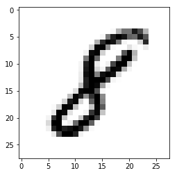
Visualizing a sample:

image_index = 7777 
print(Y_train[image_index]) 
# The label is 8
plt.imshow(X_train[image_index], cmap='Greys')

Output:

Little Preprocessing

# Reshaping the images, so that they can be fed into a model
X_train = X_train.reshape(X_train.shape[0],28,28,1)
X_test = X_test.reshape(X_test.shape[0],28,28,1)

# normalizing again after reshaping
X_train = X_train/255
X_test = X_test/255

Convolutional Neural Networks

Theory
Convolutional neural networks (CNN) is a special architecture of artificial neural networks, proposed by Yann LeCun in 1988. CNN uses some features of the visual cortex. One of the most popular uses of this architecture is image classification.
A convolutional neural network is not very difficult to understand. An input image is processed during the convolution phase and later attributed a label.

This is the basic architecture of CNN:

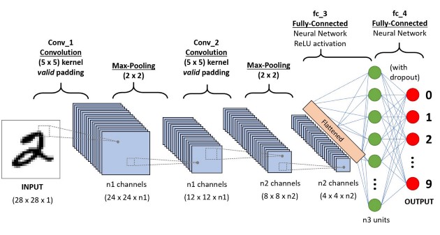
Img src: Link

An image is composed of an array of pixels with height and width. A grayscale image has only one channel while the color image has three channels (each one for Red, Green, and Blue). A channel is stacked over each other. Each pixel has a value from 0 to 255 to reflect the intensity of the color. For instance, a pixel equals to 0 will show a white color while pixel with a value close to 255 will be darker.

For example:
This is what we see

And this is what the computer sees

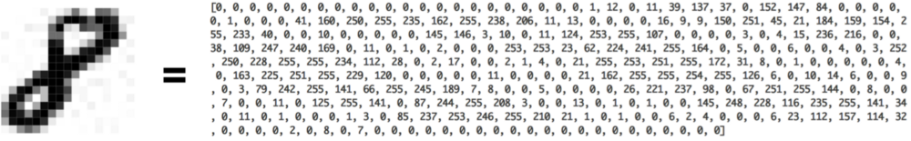
Img src: Link

Components of Convnets
There are four components of a Convnets

1. Convolution
2. Non Linearity (ReLU)
3. Pooling or Sub Sampling
4. Classification (Fully Connected Layer)

The Convolution layer is always the first.
You must have studies the concept of convolution in a higher mathematics class. Well, this is very much the same.

The purpose of convolution here is to extract the features of the object on the image locally and thereby reduce its dimensionality.
It means the network will learn specific patterns within the picture and will be able to recognize it everywhere in the picture.
Convolution is element-wise multiplication.The computer will scan a part of the image, usually with a dimension of 3x3 and multiplies it to a filter. The output of the element-wise multiplication is called a feature map.This step is repeated until all the image is scanned.
Due to the fact that pixels are only related with the adjacent and close pixels, convolution allows us to preserve the relationship between different parts of an image.

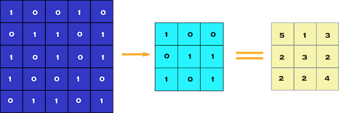
Img src: Link

The network will consist of several convolutional networks mixed with nonlinear and pooling layers. When the image passes through one convolution layer, the output of the first layer becomes the input for the second layer. And this happens with every further convolutional layer.

Non-Linearity layer(ReLU)
At the end of the convolution operation, the output is subject to an activation function to allow non-linearity. The usual activation function for convnet is the Relu. All the pixel with a negative value will be replaced by zero.

The pooling layer follows the nonlinear layer. It works with the width and height of the image and performs a downsampling operation on them. As a result, the image volume is reduced.
This means that if some features (as for example boundaries) have already been identified in the previous convolution operation, then a detailed image is no longer needed for further processing, and it is compressed to less detailed pictures.
The steps are done to reduce the computational complexity of the operation. By diminishing the dimensionality, the network has lower weights to compute, so it prevents overfitting.

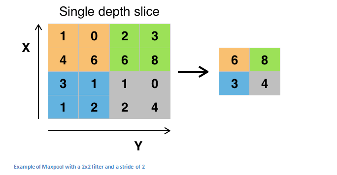
Img src:Link

This is an example of Max Pooling, wherein the maximum value of the feature map is taken as the output.

Our final layer is the fully connected layer, which takes the output information from convolutional networks.
Attaching a fully connected layer to the end of the network results in an N-dimensional vector, where N is the number of classes from which the model selects the desired class.

Implementation of the CNN model

1. Model Construction
   Code:

model = Sequential()

model.add(Conv2D(28,(3,3),strides=(1,1),input_shape=X_train.shape[1:]))
model.add(Activation("relu"))
model.add(MaxPooling2D((2,2)))

model.add(Flatten()) # flattens the input
model.add(Dense(128))
model.add(Activation('relu'))
model.add(Dropout(0.2))
model.add(Dense(10))
model.add(Activation('softmax'))

Layer 1: Conv2D (Convolution layer)
Arguments:

• filters : Denotes the number of Feature detectors.
• kernel_size : Denotes the shape of the feature detector. (3,3) denotes a 3 x 3 matrix.
• strides = controls how many units the filter shifts
• input shape : standardizes the size of the input image
• padding(optional argument) : used to control the dimensionality of the convolved feature with respect to that of input. It can be either valid (also called zero padding/no padding) which reduces the dimension or same which preserves or increases the dimension.

The dimension of the output of a convolution layer is :
o = ((N - K + 2P)/s) + 1
where,
N is the width and height of the input image
K is the kernel size
P is the padding(same or valid).
s is the stride

Layer 2 : Activation layer (ReLU)
Rectified Linear Unit is an activation function which helps in breaking the linearity and helps in modeling the response variable(class label)

Layer 3 : Pooling layer (Max Pooling used here)
Arguments:
pool_size : the shape of the pooling window.

Layer 4 : Fully connected layer (Dense layer)

Layer 5 : Dropout layer
This layer “drops out” a random set of activations in that layer by setting them to zero, thereby making the model robust and preventing overfitting.

2. Model Training

# model compilation
model.compile(optimizer='adam', 
              loss='sparse_categorical_crossentropy', 
              metrics=['accuracy'])
              
# model fitting
history = model.fit(x=X_train,y=Y_train, epochs=10)
history

3. Model Evaluation
   Let's evaluate the performance of our model on test data

model.evaluate(X_test, Y_test)

Output:
Loss - 0.05
Accuracy - 98.73%
This is an impressive result, even though model was trained for just 10 epochs.

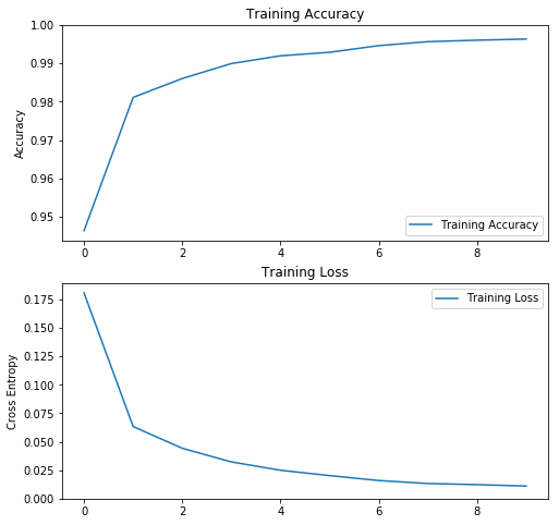
Visualizing loss and accuracy

acc = history.history['acc']
loss = history.history['loss']

plt.figure(figsize=(8, 8))
plt.subplot(2, 1, 1)
plt.plot(acc, label='Training Accuracy')
plt.legend(loc='lower right')
plt.ylabel('Accuracy')
plt.ylim([min(plt.ylim()),1])
plt.title('Training Accuracy')

plt.subplot(2, 1, 2)
plt.plot(loss, label='Training Loss')
plt.legend(loc='upper right')
plt.ylabel('Cross Entropy')
plt.ylim([0,max(plt.ylim())])
plt.title('Training Loss')
plt.show()

Output:

Why ConvNets Work so well?

• ConvNets are hugely popular because of their architecture — the best thing is that there is no need for feature extraction. The system learns to do feature extraction and the core concept of CNN is, it uses convolution of image and filters to generate invariant features that are passed onto the next layer. The features in the next layer are convoluted with different filters to generate more invariant and abstract features and the process continues till one gets final feature/output.
• A ConvNet is able to successfully capture the Spatial and Temporal dependencies in an image through the application of relevant filters. The architecture performs a better fitting to the image dataset due to the reduction in the number of parameters involved and the re-usability of weights. In other words, the network can be trained to understand the sophistication of the image better.

Check out this video to understand how neural networks think.

Final Takeaway

It is the automated feature extraction that makes CNNs highly suited and accurate for computer vision tasks such as object/image classification. The main advantage of CNN compared to its predecessors is that it automatically detects the important features without any human supervision(no pun intended!).

Again, do share if you liked the content:)