
Get this book -> Problems on Array: For Interviews and Competitive Programming
In this article, we are going to explore D’Esopo-Pape Algorithm, a single source shortest path algorithm proposed by D’Esopo and Pape in 1980. This is an efficient alternative to the famous Dijkstra's Algorithm, but has an exponential time complexity in the worst case.
📝Table of contents:
- What is D’Esopo-Pape Algorithm?
- D’Esopo-Pape Algorithm under the hood
- Complexity of D’Esopo-Pape Algorithm
- Application of D’Esopo-Pape Algorithm
- Questions to ponder
- Reference
❓1. What is D’Esopo-Pape Algorithm?
🧠First, refresh your memory on Dijkstra's Algorithm
To begin with, Dijkstra's Algorithm is a famous single source shortest path algorithm. What does a single source shortest path algorithm mean? Visualize a loosely connected graph with 5 vertexes
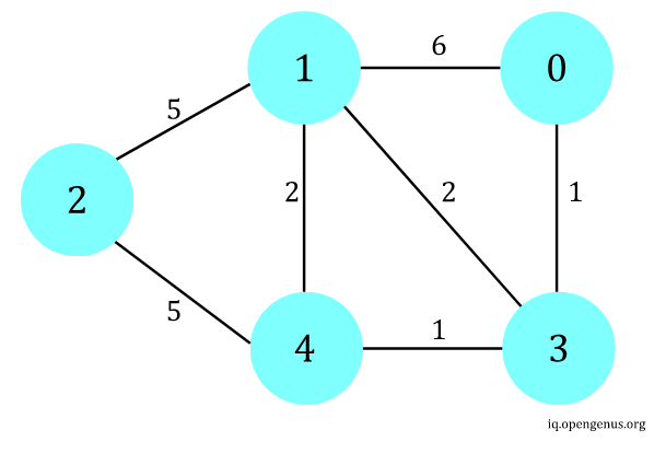
Figure 1
For Dijkstra to work, a source must first be specified, (let's assume source = vertex 0, hence single source). After running Dijkstra, the shortest paths from source to all vertexes are calculated and one can traversal from vertex 0 to every other vertexes with the guaranteed shortest path. Details of Dijkstra can be found here. In a nutshell, it works by greedily choosing the next vertex with minimum cost from source to traverse (best-first scanning) and update their cost if applicable. It also assumes there are no negative weight edges. But how does it relates to our topic of the day?
❓How D’Esopo-Pape Algorithm differs from Dijkstra's?
D’Esopo-Pape Algorithm, on the other hand, does not use a greedy approach to pick the next traversal. It instead chooses the next immediately available vertex from the queue to traverse regardless of its cost (breadth-first scanning). Moreover, D’Esopo-Pape Algorithm works with graphs with negative weight edges, provided that there are no cycles with an overall negative weight[1]. However, D’Esopo-Pape Algorithm, although has a better average runtime then Dijkstra in general, has exponential runtime in some cases traversing a dense graph[2].
🚙2. D’Esopo-Pape Algorithm under the hood
🖥️Pseudocode [1]
D’Esopo-Pape(src):
    distance[v] = infinity for each vertex v
    distance[src] = 0

    previous[v] = NULL for each vertex v

    // Initialize a double-ended queue, deque should have constant runtime
    // inserting and deleting from front and back
    de = deque()
    de.pushback(src)

    while de is not empty:
        // Extract the next available vertex from the queue
        v = de[1]
        de.popfront()

        for each neighbor u of v:
            alt_cost = distance[u] + weight of edge u -> v
            if alt_cost < distance[v]:
                distance[v] = alt_cost
                previous[v] = [u]

                // insert elements back into the queue
                if v is not in the queue and has never joined queue previously:
                    // append to the back of queue
                    de.pushback(v)

                else if v is not in the queue and has joined queue previously:
                    // append to the front of queue
                    de.pushfront(v)
As shown in the comments above, D’Esopo-Pape Algorithm uses deque instead of normal queue which maintains a constant time operation for pushback() and pushfront(). At each loop, the first element in deque is popped instead of choosing the vertex with the lowest cost. After updating the cost to vertex v, v would be appended (front or back) to deque subjected to the conditionals. It is quite similar to Dijkstra's Algorithm with a few tweaks.
👀Visualize D’Esopo-Pape Algorithm
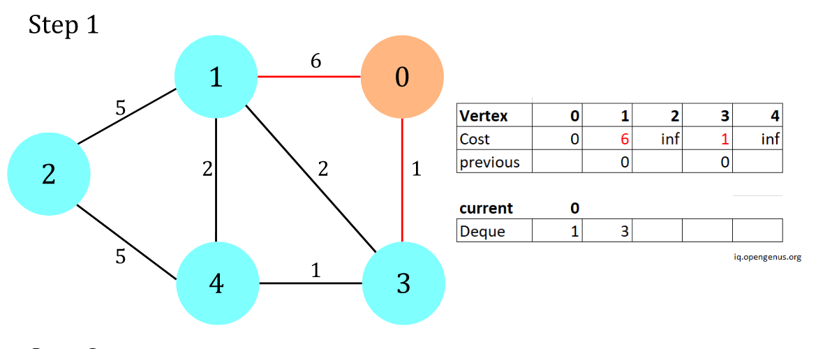
Figure 2
First start by vertex 0, and put 1, 3 into the deque, update the cost and previous array accordingly.
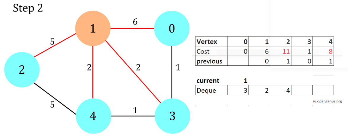
Figure 3
Traverse vertex 1 and add its unvisited neighbors 2, 4 onto the back of the deque.
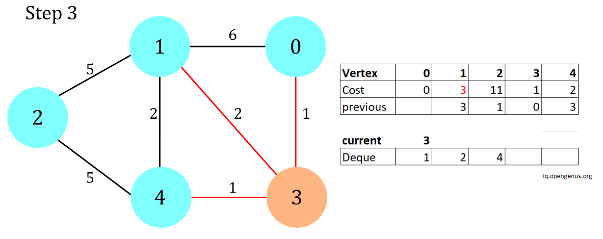
Figure 4
Traverse vertex 3 and add its visited neighbour (vertex 1) to the front of the deque.
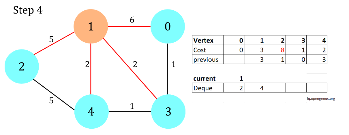
Figure 5
Continue...
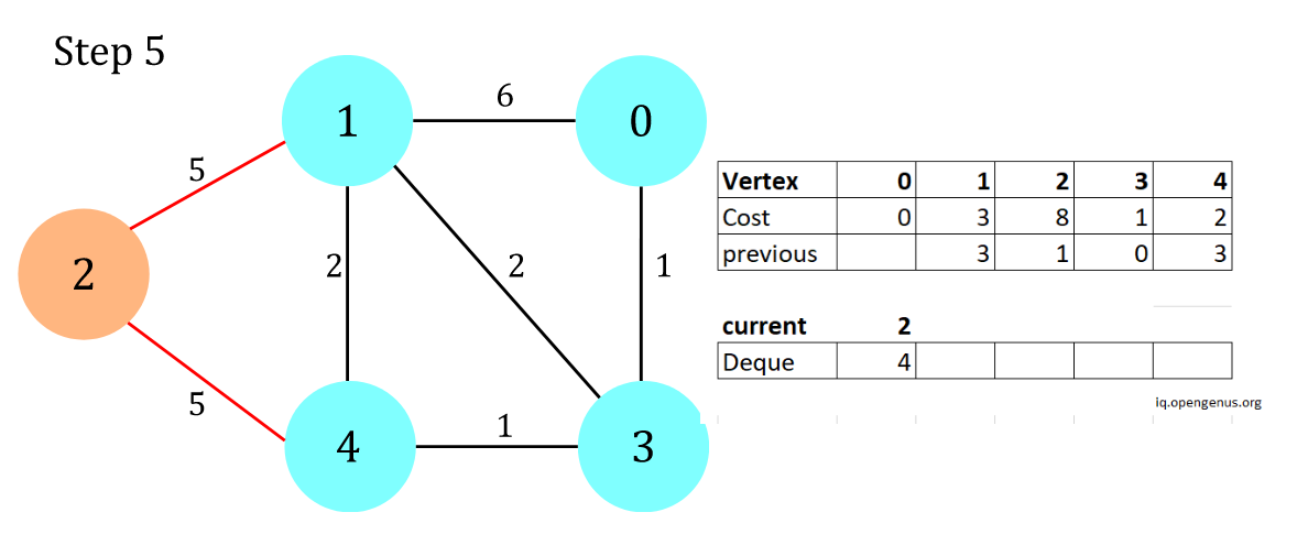
Figure 6
If there is no vertex's cost lower than the alterative cost from vertex 2, no elements would be added to the deque.
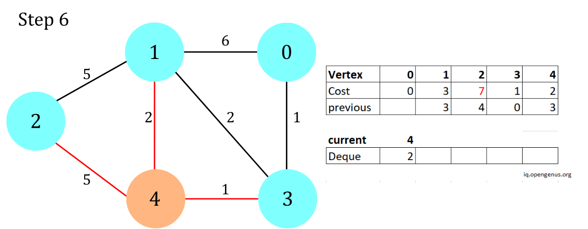
Figure 7
Continue...
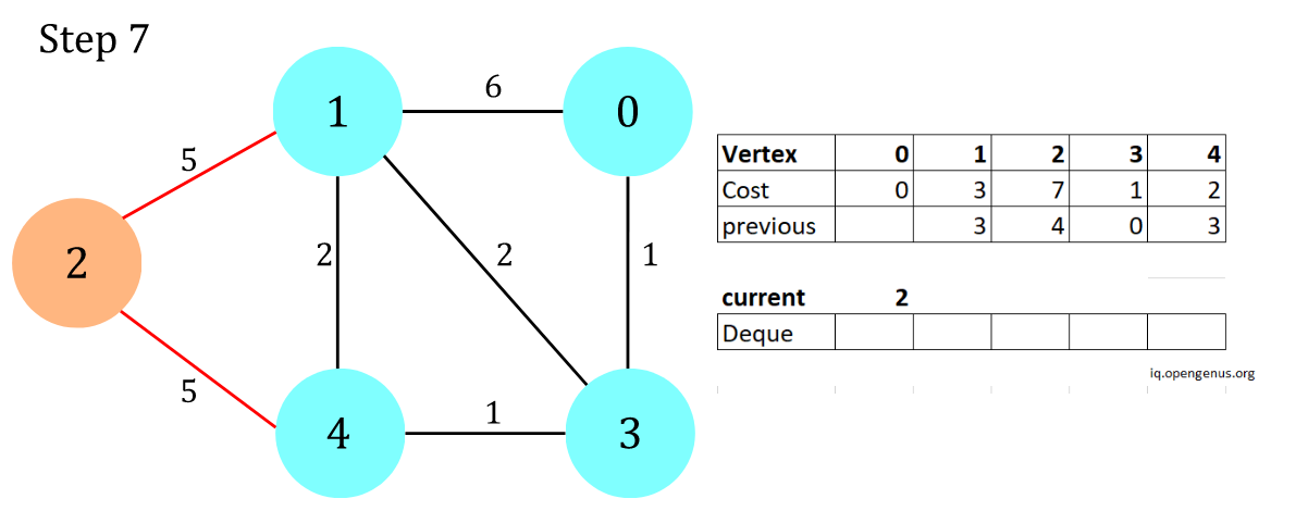
Figure 8
Finally the algorithm finishes by clearing the deque with no vertex to add to it.
🖥️Code implementation in Python
Below shows the implementation of D’Esopo-Pape with respect to the graph shown in Figure 1.
from collections import deque

class Graph:
    """
    This is the init method who initializes the field of this class,
    initialize the num_of_vertexes to the number of vertexes as input from argument
    initialize the num_of_edges to zero
    initialize the adj_list G and set the key as 0 to num_of_vertexes - 1 (from vertex)
        and value as a tuple (to_vertex, edge weight)
    """
    def __init__(self, num_of_vertexes):
        self.num_of_vertexes = num_of_vertexes
        self.num_of_edges = 0
        self.G = {v: list() for v in range(num_of_vertexes)}


    def add_edge(self, src, dest, w, bi=False):
        """
        This method allows addition of edge into graph by mutating the adj_list,
        everytime a source -> destination with weight, the adj_list is mutated such that
        (destination, weight) is added into key = source. bi = True means it is added
        in two directions, source -> destination with weight and destination -> source with weight

        Parameter:
            src: an int, source vertex
            dest: an int, destination vertex
            w: an int, weight, cost required to traverse from source not to destination vertex
            bi: a boolean, whether the edge is undirected, default to False for directed edge

        Return:
            None
        """
        if bi:
            self.G[src].append((dest, w))
            self.G[dest].append((src, w))
        else:
            self.G[src].append((dest, w))


    def run_DEP(self, src):
        """
        This method runs D'Esopo-Pape algorithm it is a breadth-first algorithm

        Parameter:
            src: an int, source from which all vertexes cost is connected

        Return:
            cost_to_v: a hashmap, cost to every vertex v from src
            prev: a hashmap, previous vertex for which each vertexes is traversed
        """
        # Initialize the cost from src to each vertex to infinity
        cost_to_v = [float("inf") for v in range(self.num_of_vertexes)]

        # Initialize the previous vertex from each every vertex is reached from
        prev = [None for v in range(self.num_of_vertexes)]

        de = deque()

        #  A list to decide if vertexes are in this array
        # -1 at ith index means vertex i has never joined the queue
        #  0 at ith index means vertex i has joined the queue but currently not in queue
        #  1 at ith index means vertex i has joined the queue currently
        memo = [-1] * self.num_of_vertexes
        cost_to_v[src] = 0
        de.append(src)

        # Initialize an array for visited
        while len(de) > 0:
            # Get the next vertex
            u = de.popleft()
            memo[u] = 0

            for (v, w) in self.G[u]:
                # Modify the cost_to_v only if there is a shorter path
                alt_cost = cost_to_v[u] + w
                if alt_cost < cost_to_v[v]:
                    cost_to_v[v] = alt_cost
                    prev[v] = u

                    if memo[v] == -1:
                        # if the vertex v has never joined the queue, append to back
                        memo[v] = 1
                        de.append(v)
                    elif memo[v] == 0:
                        # if the vertex v has joined the queue before, append to front
                        memo[v] = 1
                        de.appendleft(v)

        return cost_to_v, prev


if __name__ == "__main__":

    g = Graph(5)
    g.add_edge(0, 1, 6, bi=True)
    g.add_edge(1, 2, 5, bi=True)
    g.add_edge(4, 2, 5, bi=True)
    g.add_edge(3, 4, 1, bi=True)
    g.add_edge(0, 3, 1, bi=True)
    g.add_edge(1, 3, 2, bi=True)
    g.add_edge(1, 4, 2, bi=True)

    for src, neigh in g.G.items():
        print(src, ": ", neigh)

    cost_to_v, prev = g.run_DEP(0)

    print(cost_to_v)
    print(prev)
    print()
⌛💫3. Complexity of D’Esopo-Pape Algorithm
⌛Time complexity and best use case
Intuitively, D’Esopo-Pape Algorithm is more efficient then Dijkstra's Algorithm (Priority Queue implementation) in most spare graph traversal since the latter requires maintenance of min binary heap with O(log V) runtime for extract_min and decrease_cost functions, but the former only uses a deque to pop and append vertexes with constant runtime.
Note that each vertex would enter and leave the deque several times, and that increases the runtime of D’Esopo-Pape, but in a spare graph where each vertexes enters the deque in constant amount of time, the benefit of re-entering with constant push and pop runtime for D"Esopo-Pape would outweigh the logarithmic runtime for maintaining a heap with each vertex traversed once only. Therefore D’Esopo-Pape performs more efficiently in single-source shortest path calculation than Dijkstra. Ideally D’Esopo-Pape is best used in spare real-life network where number of vertexes are orders of magnitude larger than average nodal degree (between 2 to 3), which is found to outperform all other similar algorithms [2].
However, one must always consider the worst case. It happens when applying D’Esopo-Pape to a dense graph with a particular edge weight setting. In a dense graph, average nodal degree is close to the number of vertexes, upon traversing every vertex, all its neighbours would be relabelled, and so on for all the secondary neighbours. Simply put, from source u, it could potentially be relabelled O(V) times from all first-degree neighbours; from second-degree neighbours there are O(V^2) ways to "resurrect" u; from third-degree neighbours there are O(V^3) ways; ....; all the way till (V-1)-degree neighbours with O(V^V) numbers of ways to re-examine the source. The total time complexity of examinating a vertex is exponential, and thus the worst time complexity of D’Esopo-Pape is exponential -- O(V^V).
💫Space complexity
Referring to the pseudocode, Space complexity of D’Esopo-Pape should be O(V) since for all arrays which store 1. cost and 2. previous vertex traversed would at most occupy O(V) space with each of them individually stores at most all vertexes at any iteration.
🌎4. Application of D’Esopo-Pape Algorithm
-
IP routing: The graph of network connection is relatively spare, which this algorithm provides the shortest path from source router to all other routers in the network.
-
Flight path scheduling: This algorithm can calculate the shortest path costed from source airport to all other airports. Given the fact that airport flight paths are not densely connected, it runs optimally by planning the paths with shortest cost (time, fuel or whatever parameter one desires) from source to any destination.
-
Social networking application: Online social networking graphs are spare, which the number of users (vertexes) are orders of magnitude larger than the average nodal connections between users (edges). This algorithm can be used to calculate the shortest path from a user to any other user in the graph, and determine the degree of connection.
-
Map route finding: Maps destinations are spare since every city is not connected to all other cities. Upon calculations from source to certain destination, this algorithm can be deployed to find the shortest cost path (time, fuel or whatever parameter one desires).
💭5. Questions to ponder
Which real-life scenario is D’Esopo-Pape Algorithm NOT suitable?
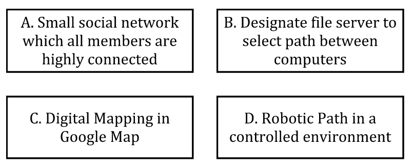
(Answer at the end of this essay)
📚6. Reference
[1] Lecture 6: Shortest Path Algorithms: (Part I) by Prof. Krishna R. Pattipati, page 33-34, https://cyberlab.engr.uconn.edu/wp-content/uploads/sites/2576/2018/09/Lecture_6.pdf
[2] "A note on finding shortest path trees", Aaron Kershenbaum, 1981, NetworksVolume 11, Issue 4 p.399-400
Answer: A. Small social network with highly connected members are a great representation of a dense graph in real life, which D’Esopo-Pape Algorithm may have exponential time complexity. Other options are a natrual spare graph which average nodel connections are orders of magnitude less than the number of vertexes, thus suitable to apply [2].