Exponential Linear Unit (ELU) is an activation function which is an improved to ReLU. We have explored ELU in depth along with pseudocode.

Table of contents:

1. Introduction
2. Mathematical Definition of ELU
3. Learning Using the Derivative of ELU
4. Pseudocode of ELU

Prerequisite: Types of activation functions

Introduction

Convolutional neural networks work by establishing layers of nodes, which are basically centers of data processing that communicate or work together towards learning. So, nodes get inputs from other nodes or from the system, and send outputs to other nodes or for the whole network. Engineers do this by employing activation functions, which basically define the output of a node given a certain input and other parameters.There are multiple kinds of activation functions and different ways for activation for each type, but this article will focus on Exponential Linear Unit (ELU) Activation function.

Mathematical Definition of ELU

The mathematical definition of this algorithm is:

Given an input x, the output f(x) is such that:

f(x) = x, for x> 0
f(x) = 𝜇(exp(x)- 1), for x ≤ 0

f'(x) = 1, for x>0
f'(x) = 𝜇(exp(x)), for x ≤ 0

where 𝜇 > 0

Exponential Linear Units are different from other linear units and activation functions because ELU's can take negetive inputs. Meaning, the ELU algorithm can process negetive inputs(denoted by x), into usefull and significant outputs.

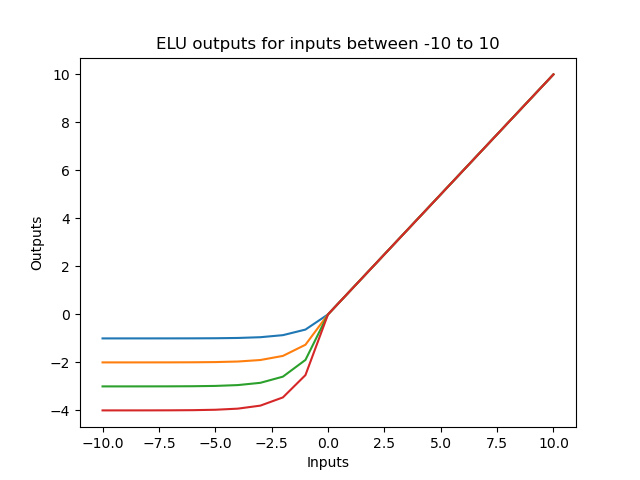
If x keeps reducing past zero, eventually, the output of the ELU will be capped at -1, as the limit of exp(x) as x approaches negetive infinity is 0. The value for 𝜇 is chosen to control what we want this cap to be regardless of how low the input gets. This is called the saturation point. At the saturation point, and below, there is very little difference in the output of this function(approximately 𝜇), and hence there’s little to no variation(differential) in the information delivered from this node to the other node in the forward propagation.

In contrast to other linear unit activation functions, ELUs give negative outputs(i.e activations). These allow for the mean of the activations to be closer to 0, which is closer to the natural gradient, so the outputs are more accurate. This reduced difference in the unit gradient and the natural gradient makes learning more efficient as the training of the model will hence converge faster.

Learning Using the Derivative of ELU

Convolutional Neural Networks employs the use of back propagation algorithms during learning. Basically, the algorithm is going to go back into the neurons to learn the historical steps taken to reach an outcome.

Forward propagation is the steps taken to reach an outcome from input to output. The error of the algorithm is calculated by the (actual value - the outcome) sqaured / 2. Essentially, what back propagation does is to go back and optimize the weights of each node. It does this by finding the effect on the error when you change the weights by a small value(i.e d(error)/d(weight)).So for the node that uses the ELU activation function, the differential of the ELU is needed and will be used in reference to the differential of the output error.

Now let's focus on the derivative function of ELU.

f'(x) = 1, for x>0
f'(x) = 𝜇(exp(x)), for x ≤ 0

for x ≤ 0,
f(x) = 𝜇(exp(x)-1)
hence,
f'(x) = 𝜇 * (exp(x)-1)' + 𝜇' * (exp(x)-1), Product Rule
f'(x) = 𝜇 * (exp(x)) + 0
f'(x)= 𝜇(exp(x)
futher more,
f'(x)= 𝜇(exp(x) - 𝜇 + 𝜇
f'(x) = 𝜇(exp(x) - 1) + 𝜇
therefore,
f'(x) = f(x) + 𝜇

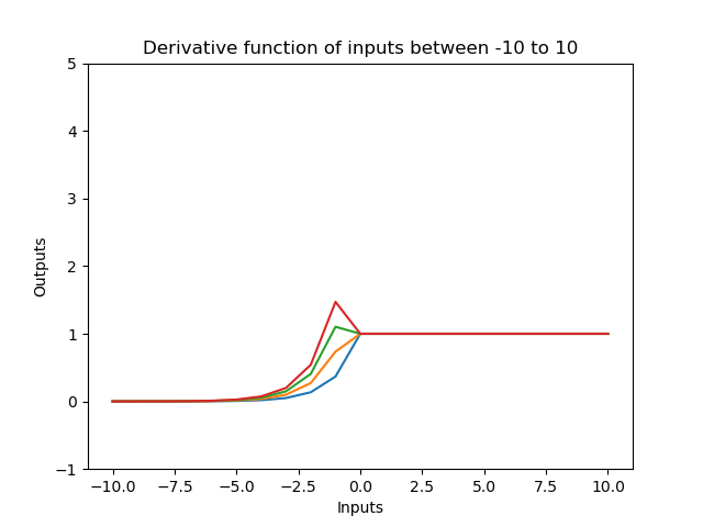
Since back propagation and forward propagation is done simultaneously, we need a function for the derivative of f(x) to have low computational cost. Since the value of f(x) and 𝜇 is already stored you can get f'(x) by finding the sum of f(x) and 𝜇 at a lower computational cost.

Pseudocode of ELU

Below is a pseudocode of the exponential linear unit activation function and the derivative function with multiple values of 𝜇.

import numpy as np
import matplotlib.pyplot as plt


def elu(x, u):
    if x >= 0:
        return x
    else:
        return u*(np.exp(x) - 1)


def elu_prime(x, u):
    if x >= 0:
        return 1
    else:
        return elu(x, u) + u


for u in range(1, 5):
    inputs = [x for x in range(-10, 11)]
    outputs = [elu(x, u) for x in inputs]
    output_prime = [elu_prime(x, u) for x in inputs]
    plt.plot(inputs, outputs)
    plt.plot(inputs, output_prime)


plt.ylim(-1, 5)
plt.title("ELU outputs for inputs between -10 to 10")
plt.title("Derivative function of inputs between -10 to 10")
plt.ylabel("Outputs")
plt.xlabel("Inputs")
plt.show()

Below is the graph representing the algorithm, as well as the derivative function.

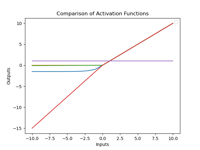
Now below is just a comparison of the ReLU, LeReLU, Swish, and Sigmoid activation functions with ELU with u = 1.5.

import numpy as np
import matplotlib.pyplot as plt


def elu(x, u):
    if x >= 0:
        return x
    else:
        return u*(np.exp(x) - 1)


def elu_prime(x, u):
    if x >= 0:
        return 1
    else:
        return elu(x, u) + u


def ReLu(x):
    if x < 0:
        return 0
    else:
        return x


def LRelu(x):
    if x < 0:
        return 0.01 * x
    else:
        return x


def PRelu(x, u):
    if x < 0:
        return u*x
    else:
        return x


def softmax(x):
    y = np.exp(x)
    y_final = y / y.sum()
    return y_final


u = 1.5
inputs = [x for x in range(-10, 11)]
output_e = [elu(x, u) for x in inputs]
output_r = [ReLu(x) for x in inputs]
output_l = [LRelu(x) for x in inputs]
output_p = [PRelu(x, u) for x in inputs]
output_s = [softmax(x) for x in inputs]
plt.plot(inputs, output_e)
plt.plot(inputs, output_r)
plt.plot(inputs, output_l)
plt.plot(inputs, output_p)
plt.plot(inputs, output_s)



plt.title("Comparison of Activation Functions")
plt.ylabel("Outputs")
plt.xlabel("Inputs")
plt.legend()
plt.show()

With this article at OpenGenus, you must have the complete idea of Exponential Linear Unit (ELU).