Flattened Convolutional Neural Network

In this article, we have explored the idea of Flattened Convolutional Neural Network and the problem of conventional CNN it solves.

Table of contents:

1. Introduction to Convolutional Neural Networks
2. Problems with Conventional Convolutional Neural Networks
3. A Solution (Flattened Convolutional Neural Networks)
4. Training Flattened Convolutional Models
5. Benefits
6. Summary

Introduction to Convolutional Neural Networks

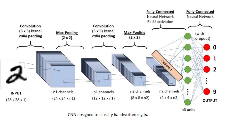
Convolutional Neural Networks (CNNs) are a class of Artificial Neural Networks that are most often used in image classification, recommender systems, natural language processing, and more. Before CNNs were in use, identifying objects in images was a very slow and sluggish process. However, CNNs now provide a simpler approach to object recognition and image classification.

They are essentially regularized versions of multilayer perceptrons. They have three layers: the convolutional (kernel) layer, the pooling layer, and the fully-connected layer. They take an input image, reduce the dimensionality of the data (in order to make the image easier to process without losing essential features which are necessary to make a good prediction), and finally, pass the resultant data to the fully-connected layer, which classifies the image based on the features extracted in the previous layers. The dimensionality of the data is reduced through the convolutional (kernel) layer and the pooling layer. Before the data is passed to the fully-connected layer, however, it is first 'flattened'. This means that the data is converted to a single, long, one-dimensional feature vector, which is in turn connected to the final classification model, or the fully-connected layer. CNNs, despite showing great promise and real world relevance, are very computationally heavy algorithms that require fast GPUs and/or servers.

Now that we have a brief understanding of conventional Convolutional Neural Networks, it is time to discuss a few ways in which they can be improved by drawing attention to some of their biggest shortcomings.

Problems with Conventional Convolutional Neural Networks

Conventional Convolutional Neural Networks exhibit high redundancy. The filters in the network often have similar patterns, and there is often more noise than distinct and distinguishable features. This has a negative impact on how well the network can learn, and also calls for unnecessary computations during feed-forward passes as well as back propagation. Since CNNs are computationally demanding, one way to speed up the evaluation process is to reduce the number of parameters in the network representation. Considering the fact that CNNs in the real world require a very large number (sometimes, hundreds) of filters in each layer and usually consist of three to five convolutional (kernel) layers, finding the most essential features with smaller parameters entails a significant gain in overall performance, both in terms of time as well as memory.

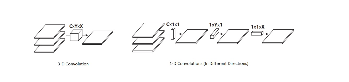
Thus, we will now take a similar approach in reducing the redundancy of the filters in Convolutional Neural Networks. We achieve this (while training the model) by separating the standard three-dimensional convolution filters into three consecutive one-dimensional filters: lateral, vertical as well as horizontal. We'll find similar if not higher levels of accuracy on popular datasets when compared to the baseline network, which has about ten-times as many parameters.

A Solution (Flattened Convolutional Neural Networks)

On training flattened networks (that consist of a consecutive sequence of one-dimensional filters across all directions in three-dimensional space), researchers Jonghoon Jin, Aysegul Dundar and Eugenio Culurciello found that they were able to obtain performance comparable to that of conventional Convolutional Neural Networks without much loss in accuracy, despite being about two times faster during feed-forward passes owing to the significant reduction in the number of learning parameters. Let us have a look at how this is implemented mathematically.

Weights in Convolutional Neural Networks can be described as four-dimensional filters:

where C is the number of input channels, X and Y are the spatial dimensions of the filter, and F is the number of filters (or output channels).

Convolution (for each channel output) requires a filter:

and is described as:

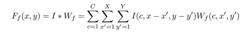
^Expression (1)
assuming a stride of one where 'f' is an index of the output channel,

is the input map, and N and M are the spatial dimensions of the input.

Now, for us to be able to accelerate multi-dimensional convolution, we have to apply filter separation. Assuming that the rank of the filter Wf is one, we can separate the unit rank filter W'f into the cross products of three one-dimensional filters as illustrated below:

W'f = αf × βf × γf
where:
αf -> Lateral Filter
βf -> Vertical Filter
γf -> Horizontal Filter

We must note that the intrinsic rank of the filter Wf is higher than one practically. We can also restrict connections in the receptive fields so that the model can learn 1-D separated filters when trained. Thus, when applied to Expression (1), a single layer of convolutional neural networks is modified to:

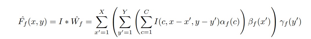
Keeping these changes in mind, we find that the number of parameters to calculate each feature map decreases from XYC to X+Y+C, and the total number of the operations needed decreases from MNCXY to MN(C+X+Y). As we will see below, this reduction in the number of parameters significantly reduces the computational load and speeds up the overall process.

Training Flattened Convolutional Models

As discussed above, the key differentiating factor between a standard (baseline) model and a flattened model is that in flattened models, we use CNNs that are constructed with one-dimensional filters. The lateral (L) filters first perform convolution across channels like mlpconv (convolution layer with a 1x1 convolution kernel) in the network. Then, vertical (V) and horizontal (H) filters, whose filter sizes are Yx1 and 1xX in space respectively, perform convolution on each channel. Once we have described the final structure of the model (during the training phase), there is no requirement for any post-processing or fine tuning. As we saw earlier, we restricted the connections in the receptive field to make the model learn 1-D separated filters, or equivalently, a rank-one 3-D filter (not accounting for biases).

Researchers Jonghoon Jin, Aysegul Dundar and Eugenio Culurciello found that replacing filters having dimensions C×X×Y with filters having dimensions C, X and Y resulted in 2−3% accuracy drops in their experiments which were conducted on a variety of datasets. 1-D separated filters with dimensions C, X and Y contain only 5% of the parameters when compared to 3-D filters in commonly used Convolutional Neural Networks, which is a vast reduction in the total number of parameters. However, even though 5% of essential parameters can successfully predict the rest of the parameters (best case scenario), such a reduction of parameters was found to be accompanied with a loss in accuracy. In their 1-D training pipeline, they found that parameters in one set of 1-D filters were not enough to distinguish discriminate features. Moreover, they also found that removing any one direction from the LVH (Lateral-Vertical-Horizontal) pipeline caused a significant loss in accuracy, which suggested that convolutions in all directions are equally essential.

Thus, in order to make up for this loss in accuracy, the team of researchers cascaded a set of LVH (Lateral-Vertical-Horizontal) convolutional layers. On doing this, they observed that the two cascaded LVH layers performed similarly to a standard convolutional layer. Depending on the complexity of the classification problem, different numbers of LVH convolutional layers can be cascaded, thus allowing for a lot of flexibility!

Thus, with proper weight initialization, it's possible for a flattened model to obtain an accuracy comparable to that of a baseline model!

Benefits

Firstly, the reduction in the number of parameters eases computational demands.

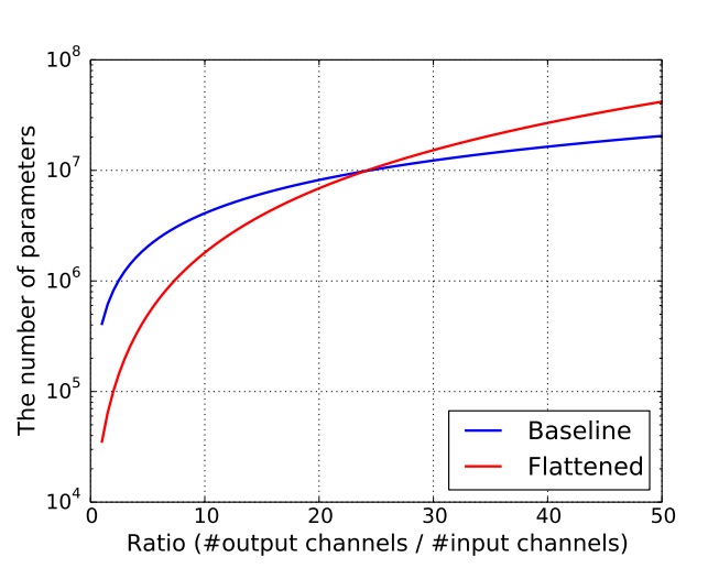
This table shows us that as long as the number of channels increases smoothly, the number of parameters should reduce greatly.

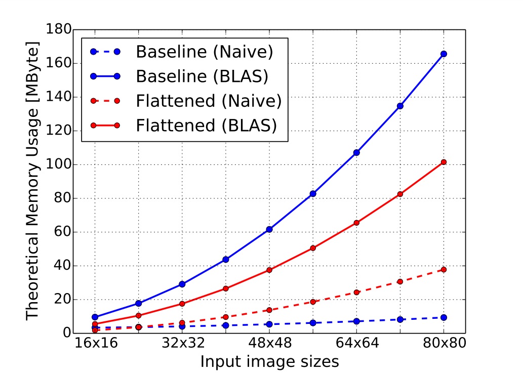
Secondly, we find that the flattened convolutional layer uses less memory than the standard convolutional layer.

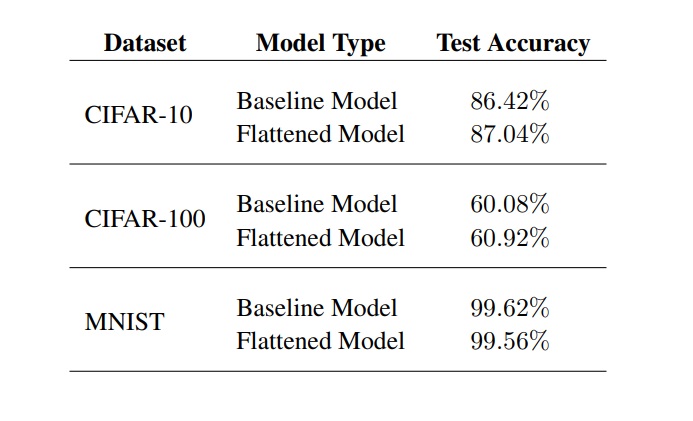
Thirdly, we find that there is little to no change when it comes to the overall accuracy when comparing the flattened model to the baseline model.

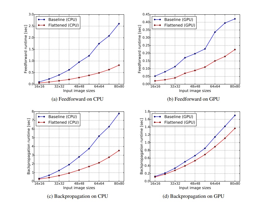
And lastly, due to the reduced number of parameters in 1-D convolutional pipelines, both feed-forward as well as back propagation computations are significantly quicker when we use flattened models instead of regular (baseline) models. It also reduces the overall time taken to train the model on both the Central Processing Unit (CPU) as well as the Graphics Processing Unit (GPU).

Summary

In this article at OpenGenus, we learned that Flattened Convolutional Neural Networks are essentially CNNs where one or more convolutional layers are converted to a consecutive sequence of one-dimensional convolutions. They allow for comparable performance with respect to conventional CNNs without a loss in accuracy, while being much quicker during the feed-forward and back propagation passes, because of the vastly reduced number of parameters. Moreover, they also do not require any post processing or manual tuning once the model has been structurally defined and trained, making them all the more sophisticated.

Thanks for reading!